

Reviewed and updated 20 July 2026
Hello!
This is the final post of this series. Today, we will be combining prior strategies into a single strategy, and analyzing its performance.
Thank you all who have recently become paid subscribers, it means the world to me.
Let’s get into it.
Recap
In Part 3, we extended the Treasury seasonality series from intra year and intra month patterns to the intra week level for the 2Y, 5Y, 10Y, and 30Y from 15 February 1977 through 4 September 2025.
The Part 3 results showed positive average Monday yield changes across all four maturities. All four remained below 5 percent after Benjamini-Hochberg adjustment of the 20 weekday-by-maturity tests. Under Bonferroni, the 2Y, 5Y, and 10Y remained below 5 percent, while the 30Y was below 10 percent rather than 5 percent. These classical t-test p-values were not tested for robustness to serial dependence or heteroskedasticity.
We translated the finding into a simple rule that shorts duration on Mondays and remains flat on other days, reporting results in yield basis points for easy DV01 scaling. Over the full sample the raw Monday short works, but performance varies by regime, with choppier results in the 1980s, solid gains through the 1990s and 2000s, a flat 2010s, and renewed strength in the 2020s.
A small implementation choice matters. Excluding Mondays that fall in the last two trading days of the month removes spillover from the month end flow that Part 2 documented and improves the risk profile. Full sample Sharpe lifts into the mid zero point five range and drawdowns become shallower with only a small reduction in trade count.
In the selected 2022–2025 window, the same Monday short with the month end exclusion delivers Sharpe between roughly 1.4 and 2.2 across the belly and the long end, with hit rates near sixty percent and contained drawdowns. That period was selected after the fact, so it is not a holdout test. The result sits naturally beside the month end long from earlier in the series, where the strongest gains arrive in the last few trading days, consistent with insurer and index rebalancing flows. Together they form a clean seasonal toolkit with complementary exposures.
The next step is to combine them thoughtfully, size in DV01 terms, and examine whether simple filters change the overall risk adjusted return.
As always, this is for educational purposes only and not financial advice.
Combined Strategy
We measure seasonality in basis-point changes of Treasury yields for the 2Y, 5Y, 10Y, and 30Y on daily closes from 15 February 1977 through 17 September 2025. P&L is reported as yield basis points captured; multiply by a position’s dollar DV01 for a first-order dollar approximation. This keeps tenor comparisons scaled, but it is not an instrument-level total-return backtest.
The code first cleans and sorts the input yields, computes the daily change in yield in basis points, and builds a trading calendar that knows each day’s weekday and position within its month.
Signals come from two places:
First, weekday rules let you short or long on specific weekdays, for example a Monday short.
Second, month end rules let you go long on the last trading day and on specified offsets such as last-1 or last-2.
The code creates boolean masks for these conditions and a position series with values of +1 for long duration, −1 for short duration, and 0 for flat.
An overlap policy decides what happens if a weekday trade and a month end long coincide. With eom_wins the month end long takes precedence and the weekday signal is skipped. With dow_wins the weekday overwrites the month end. With sum_clip the signals are added and then clipped to the range from −1 to +1.
Daily P&L is computed directly from the yield change. The article backtest assumes zero cost. The companion adds simple deductions from 0.1 to 1.0 yield basis points per side as sensitivities only; they are not calibrated transaction costs for a named instrument.
The metrics table is built from two views of the same PnL series. Active-day statistics look only at days when the strategy has a position and include the trade-only mean, standard deviation, hit rate, t-statistic, and an annualized Sharpe that uses the observed trades per year. Calendar-day statistics keep the full daily timeline, which includes zeros on non-trade days, and report the calendar standard deviation, a calendar Sharpe annualized by the square root of 252, and the maximum drawdown computed on the cumulative calendar PnL. The table also reports the sample span in years, the number of calendar days with defined PnL, the number of trade days, and total cumulative PnL in basis points per 1 dollar DV01.
The calendar is constructed from the full observed history before the 17 September 2025 cutoff is applied. This prevents the partial September 2025 window from being treated as a complete month: 15 September is a Monday short, while 16–17 September are flat. The strategy still uses close-to-close changes, so a “Monday” trade captures the move from the prior close to Monday’s close. Open-to-close execution would require intraday data and a different construction.
Backtest Strategy
After playing around with a few different versions, this was the strongest combination I tried in the same sample on Sharpe and total P&L. There was no predeclared search or held-out selection period, so “best in this search” is the appropriate interpretation.
Backtest Rules
Long the last three trading days of each month.
Short duration on Mondays.
If a Monday falls within one of the last three trading days, remain long because the month-end rule takes priority.
Backtest: Full Period (1977 - 2025)
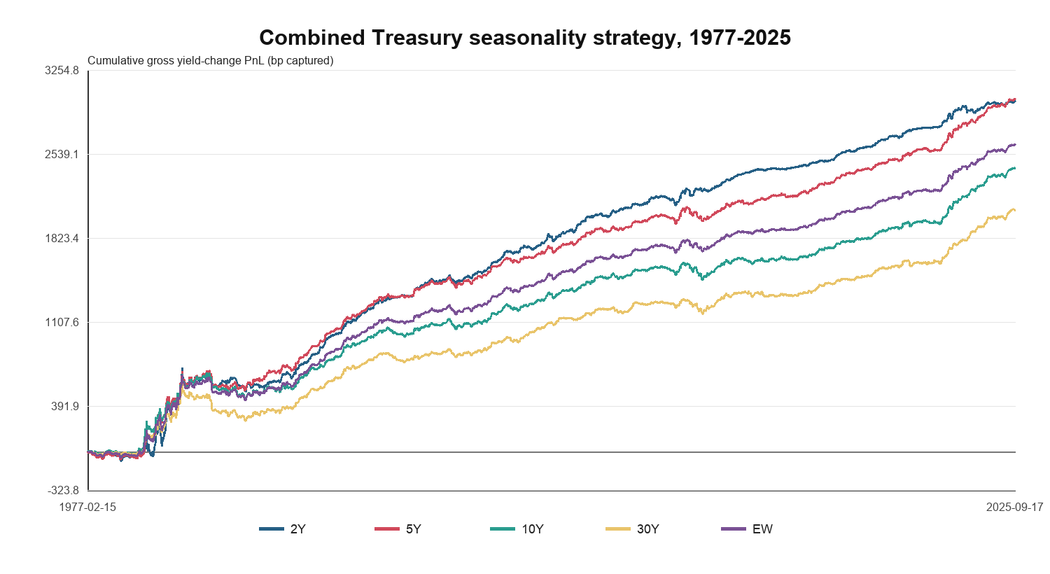
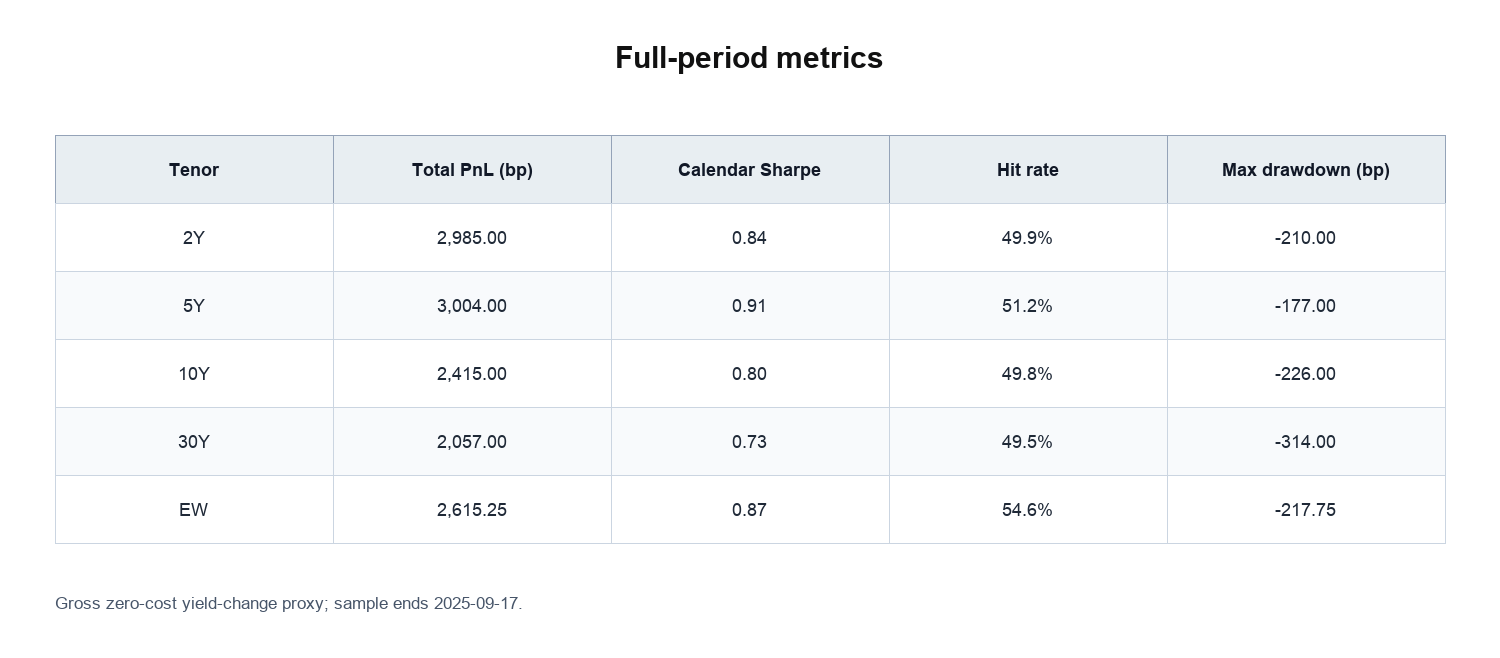
The equal-weight basket earns 2,615.25 gross yield basis points with a Sharpe near 0.87 and a maximum drawdown of about 218 basis points. A cutoff-first calendar sensitivity produces 3.50 additional gross basis points because it treats the incomplete terminal month as complete. Both specifications have the same rounded Sharpe and support the same principal gross finding.
By tenor, the 5Y is the strongest on risk-adjusted terms with a Sharpe around 0.91 and total P&L of 3,004 basis points.
The 2Y is similar in total P&L at 2,985 basis points, the 10Y reaches 2,415, and the 30Y reaches 2,057. Hit rates sit near 50 to 55 percent, so the edge comes from average gain versus average loss rather than an extremely high win rate. The cumulative P&L lines are positive over multiple decades, with the belly of the curve generally leading and the long bond lagging but still contributing.
Backtest: 2022- 2025
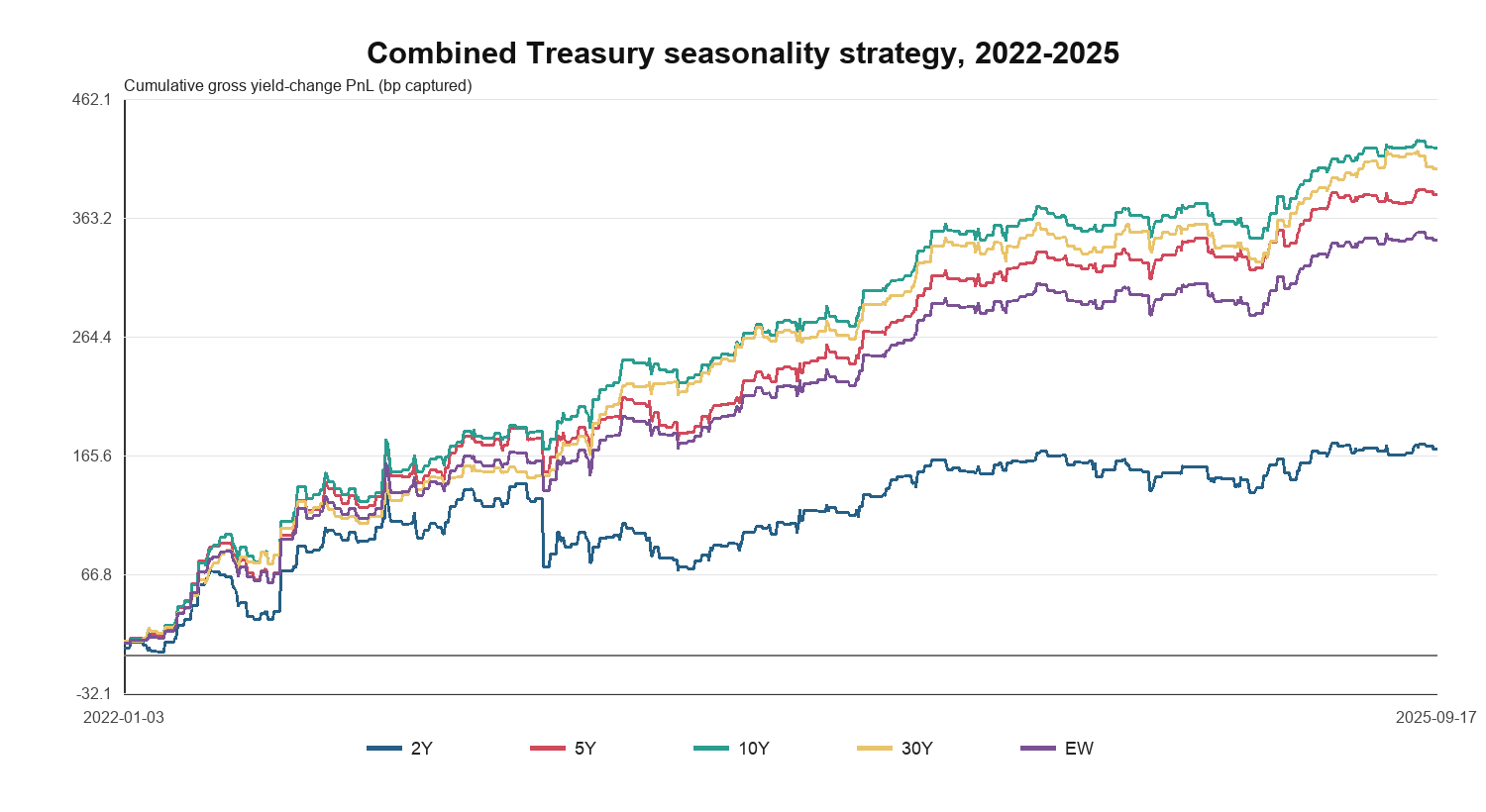
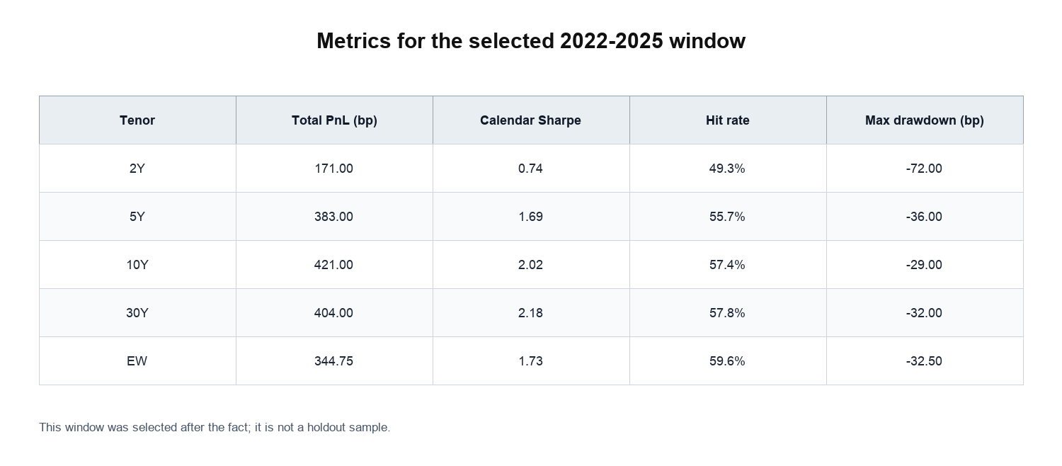
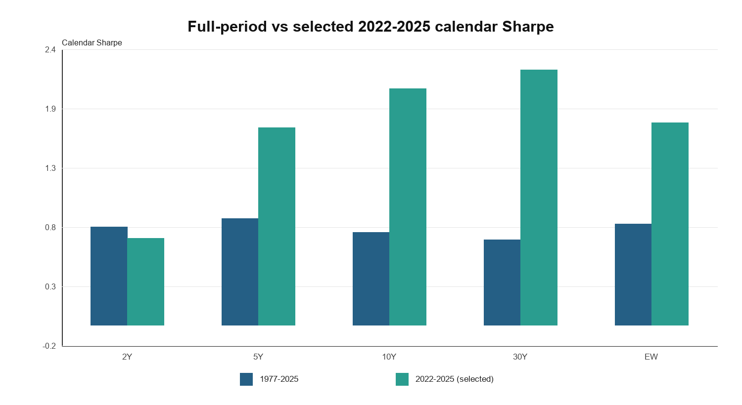
Performance is stronger in the selected 2022–2025 window. Including the prior close for the first Monday, the equal-weight basket posts a Sharpe near 1.73 with about 32.5 basis points of maximum drawdown.
The 10Y and 30Y reach Sharpe of about 2.02 and 2.18, with total P&L of 421 and 404 basis points. The 5Y also performs well with a Sharpe around 1.69, while the 2Y is positive but more muted. The cumulative charts show step-ups around month end paired with gains from Monday shorts during this window.
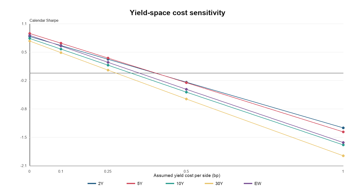
The two legs are combined here, but this analysis does not include a formal diversification decomposition or an out-of-sample comparison with each leg. The simple sensitivity also shows that costs matter: equal-weight Sharpe falls from 0.87 at zero cost to 0.25 at an assumed 0.25 yield basis points per side, and turns negative at 0.50 basis points per side. Those deductions are not estimates of a named instrument’s actual costs.