

Welcome back to another issue of Recent Academic Research!
Let’s get into it.
Momentum’s Portfolio Value, Measured in Drawdowns
Over almost a century, a dead simple rule grew about as fast as the market while cutting the worst loss nearly in half.
Momentum is the idea that rising prices tend to keep rising, and this paper tests its bluntest version on the U.S. stock market. Each month, look back one year. If the market is up, own stocks. If it’s down, sit in Treasury bills. From 1927 to 2026 the rule grew at almost exactly the market’s pace, but its worst fall from a peak was about 45% instead of 84%.
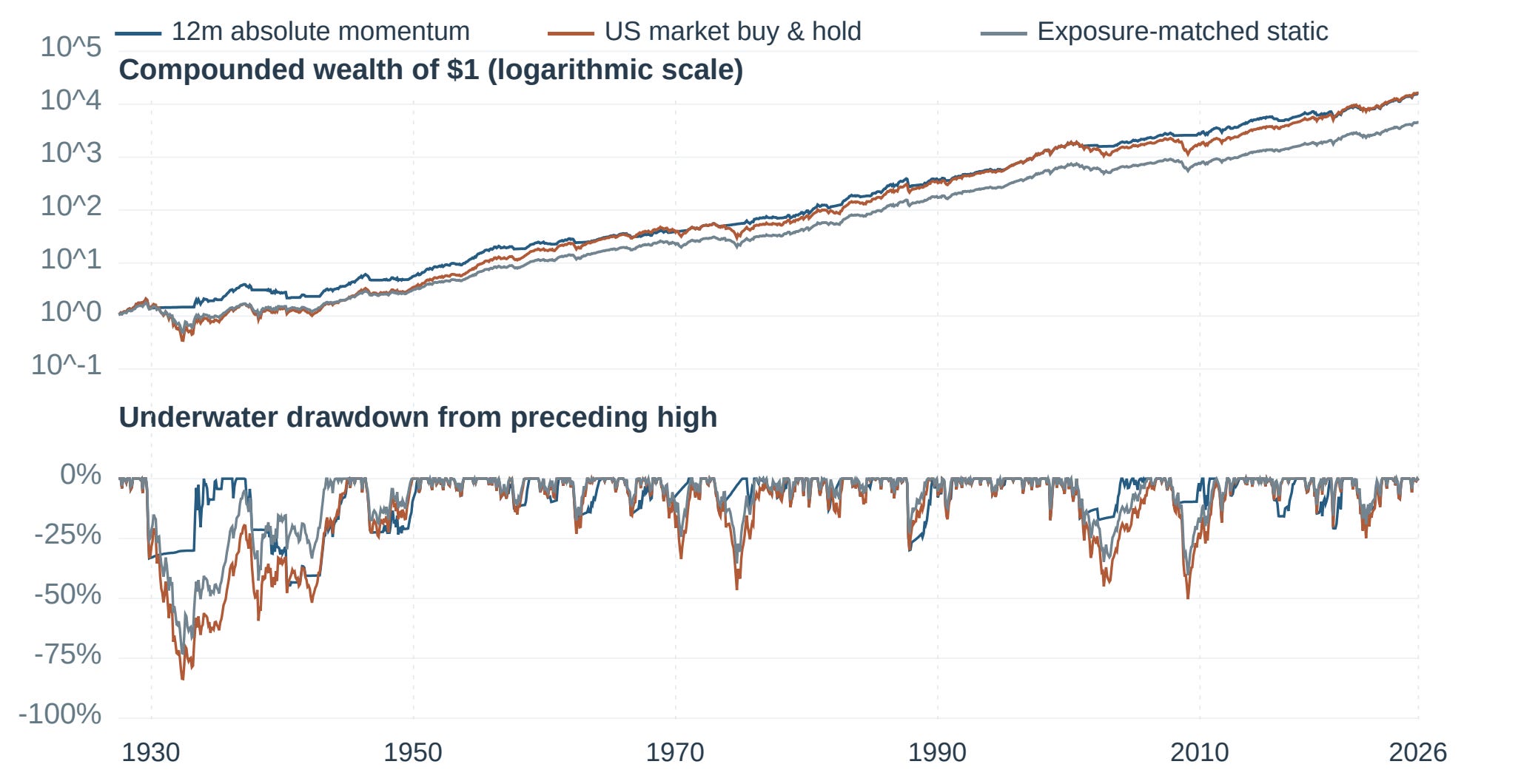
Figure 1: One dollar invested in July 1927 under three approaches: always in stocks, the one-year trend rule, and a fixed mix holding the rule’s average stock exposure. The rule ends near buy and hold, but its losses run much shallower in long slumps like the 1930s and 2008.
What’s surprising is that it isn’t just owning less stock, since a fixed mix with the same average stock exposure grew slower and fell much further. Bad markets like the 1930s or 2008 tended to unravel slowly, as news gets absorbed in stages and investors cut risk at different speeds, so a trailing signal has time to step aside. What keeps everyone from doing it is that the rule always reacts late, and fast rebounds punish it. In 2020 it sat in bills while stocks roared back from the COVID crash. This is a single-author working paper with idealized trading and a placeholder cost, and since 2010 the fixed mix did better. The lesson here isn’t to start timing. It’s that if you would bail in a crash anyway, a rule written in advance beats a panic sale, though “a momentum allocation must still earn its place in an investor’s portfolio.”
Lee, Sungkyu, Momentum as a Market Regularity: Historical Evidence, Distinct Signals, and Portfolio Value (November 07, 2026). Available at SSRN: https://ssrn.com/abstract=7707479 or http://dx.doi.org/10.2139/ssrn.7707479
Calibrating Election Markets: Primaries versus Generals
Election betting markets underprice favorites in general elections, much as racetracks always have, but in primaries they price favorites as safer than they really are.
Here is the simplest test of a betting market: Do the 80 cent candidates actually win 80% of the time? Across every head to head race on Kalshi and Polymarket since late 2023, Kirillov finds that in general elections they win more. It’s the same pattern racetracks have shown since the 1940s, because bettors overpay for long shots and that leaves the favorite too cheap. As he puts it, “favourites win more often than their prices say.” What’s convincing is that he froze his analysis and archived it before the 2026 midterms, then let the voters grade it. Polymarket favorites priced between 80% and 95% won 83 of 84 races.
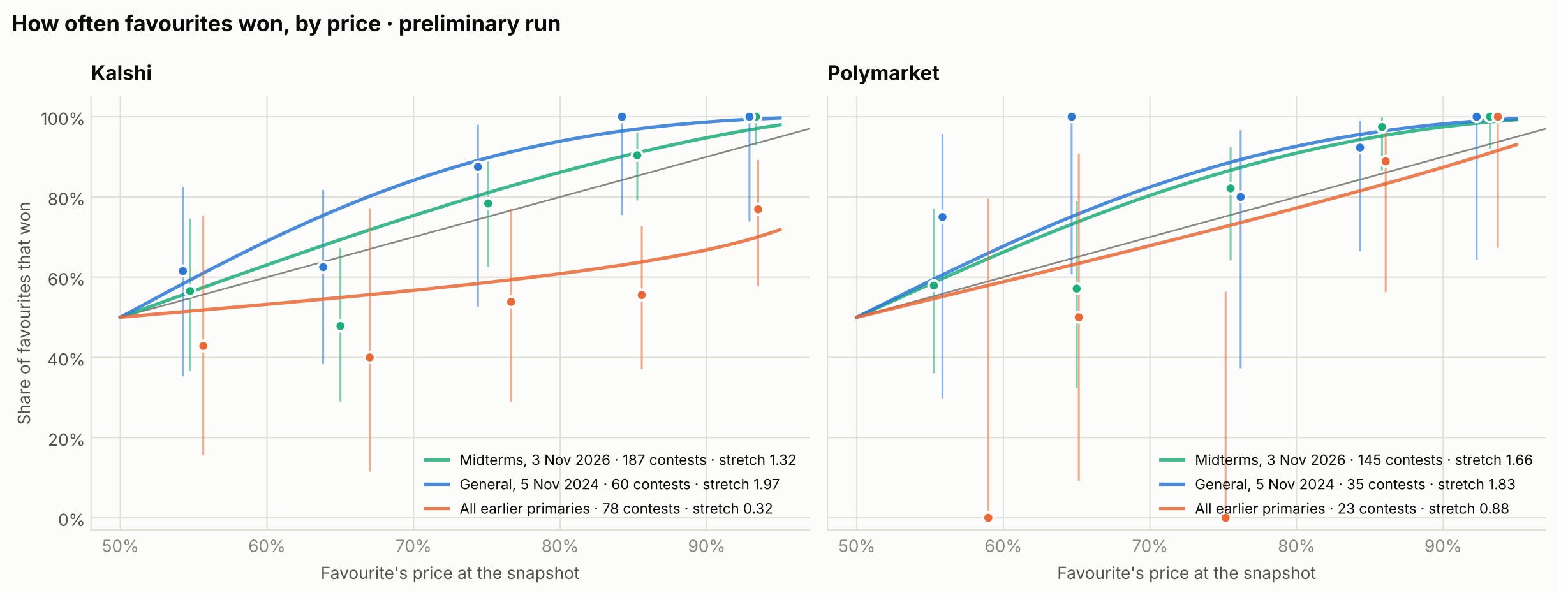
Figure 2: How often favorites actually won at each price. On the gray diagonal, prices were exactly right. Above it, as in 2024 and the 2026 midterms, favorites won more often than their prices implied. Below it, as in Kalshi’s primaries, they won less often.
Why hasn’t this been traded away? Buying every favorite earned a few percent per bet after fees, indistinguishable from luck, with cash locked up until settlement. Primaries flip the result. Kalshi’s primary favorites lost far more often than priced, plausibly because thin trading and no party label leave traders guessing with too much conviction. This rests on two general election nights and a primary finding spotted rather than tested, so treat it as a strong hint. If you check these odds before hedging a sector bet around an election, read a general election favorite as safer than its price and a primary favorite as shakier.
Kirillov, Nikita, Calibration of US Election Markets: Primaries versus General Elections on Kalshi and Polymarket, with a Pre-Registered Test on the 2026 Midterms (November 13, 2026). Available at SSRN: https://ssrn.com/abstract=7701120 or http://dx.doi.org/10.2139/ssrn.7701120
EuroCTP’s Effects on Venue Market Shares
Europe’s new consolidated tape, a single public feed of every venue’s best prices, didn’t make trading any cheaper in its first weeks, but it did move volume away from the big national exchanges.
European stocks trade on dozens of venues at once, and until September 14 there was no single public source showing the best price across all of them. If you wanted the full view, you had to buy each venue’s data feed and combine them yourself. Then EuroCTP launched one public feed of the best prices everywhere. Comparing EU stocks with UK stocks, Ewald finds that spreads didn’t budge. The market makers and big brokers who set prices already paid for the full picture, or as he puts it, “the most active participants already had a consolidated view of the market.” So the public got the view professionals had been buying for years, and the professionals carried on as before. What changed was where trading happens. Challenger venues like Cboe sat at the best price more often, brokers could now see that cheaply, and the national exchanges lost roughly 1 to 1.4 percentage points of displayed volume.

Figure 3: Change in each venue’s share of trading in EU stocks, measured against UK stocks the tape doesn’t cover. Each dot is one week, with the week before launch set to 0 and the launch at week 0. After launch, the national exchanges lose share and Cboe gains it.
Market makers also kept slightly less of each spread, a hint that slower traders now catch their stale quotes. One caveat is that this covers only 28 trading days, mostly in large stocks. The thing to watch now is whether the tape starts naming which venue has the best price, as fund industry groups already demand.
Ewald, Florian, Effects of the EuroCTP Consolidated Tape on Liquidity, Execution Quality, Fragmentation, and Venue Market Shares (October 31, 2026). Available at SSRN: https://ssrn.com/abstract=7696418 or http://dx.doi.org/10.2139/ssrn.7696418
Size Still Matters, Just Not Every Month
The small-cap premium hasn’t disappeared. It comes and goes, and you can see when it’s coming back by forecasting the stocks inside it one at a time.
The oldest idea in factor investing is that small companies beat big ones, yet the textbook bet on it (long small stocks, short big ones, the Fama French “SMB” factor) earned nothing for two decades. Azevedo, Brogaard and Weibels argue the premium isn’t dead, just moody. SMB is only a basket of stocks, so its expected return is the weighted average of its stocks’ expected returns. They trained neural networks to forecast each stock separately, then added the forecasts up using SMB’s own weights. That sum predicts next month’s SMB, and most of the signal comes from valuations read alongside whatever separates a cheap small firm from a distressed one, a distinction that averaging across firms blurs.
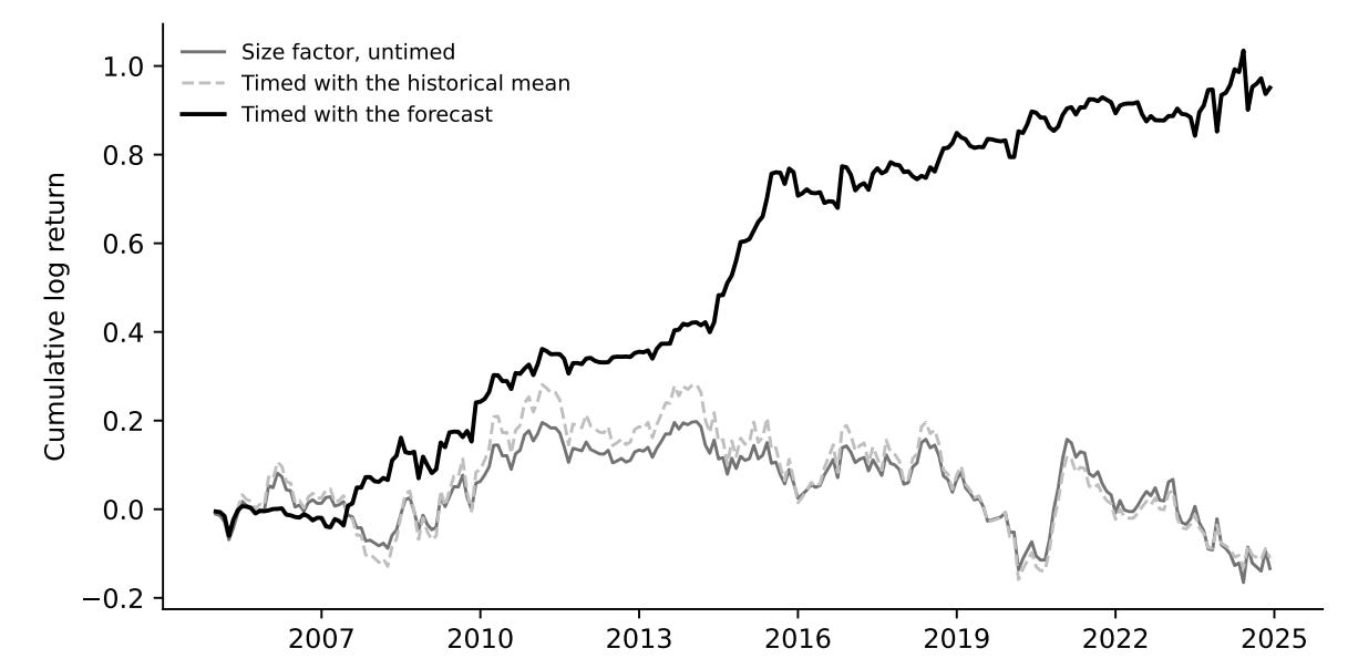
Figure 4: Twenty years of the size factor. Holding small minus big stocks went nowhere, while timing it with stock-by-stock forecasts kept compounding. These returns are before trading costs, and the paper estimates that costs cut the Sharpe ratio from 0.61 to 0.43.
It survives because small stocks digest news slowly, cost far more to trade and are pricey to short, while the drag came from small junk stocks that passive funds hold by default. Timing SMB this way earned a Sharpe ratio (return per unit of risk) of 0.43 after trading costs, and it held up across dozens of foreign markets. The catch is a thin monthly edge that leans on shorting small caps. The authors believe that passive exposure “earned none of the premium over these twenty years,” so hold it for diversification, not because you expect it to beat the S&P 500.
Azevedo, Vitor and Brogaard, Jonathan and Weibels, Sebastian, When Does Size Matter? (November 16, 2026). Available at SSRN: https://ssrn.com/abstract=7713618 or http://dx.doi.org/10.2139/ssrn.7713618
This week for paid subscribers
Paid subscribers are getting Part 1 of a two-part look at what happens when one default hits your stocks and your bonds at the same moment. The post builds a structural model where a bond issuer’s failure also pushes down every stock in the portfolio. It shows how that shared trigger takes a bad-week loss from about 2% of the portfolio to about a third, and how two holdings with no names in common end up moving together. Python code included.

Disclaimer: The content provided in this newsletter, "Alpha in Academia," is for informational and educational purposes only. It should not be construed as financial advice, investment recommendations, or an offer or solicitation to buy or sell any securities or financial instruments. Past performance is not indicative of future results. The financial markets involve risks, and readers should conduct their own research and consult with qualified financial advisors before making any investment decisions.
The interpretations, opinions, and analyses presented herein are those of the author and do not necessarily reflect the views of the original researchers, their institutions, or the full implications of the cited academic papers. While every effort is made to accurately represent the research discussed, readers should be aware that the summaries and interpretations may not capture the full scope or nuances of the original studies. The information contained in this newsletter is believed to be accurate and reliable at the time of publication, but accuracy and completeness cannot be guaranteed. The author and publisher accept no liability for any loss or damage resulting from reliance on the information provided.
This newsletter may contain links to external websites or resources. The author is not responsible for the content, accuracy, or reliability of these external sources.
By subscribing to or reading this newsletter, you acknowledge that you have read and understood this disclaimer and agree to hold the author and publisher harmless from any liability that may arise from your use of the information contained herein.