The Mechanics of Skew and Vanna: Part 1

[WITH CODE] Why is the Volatility Surface Skewed, and Can We Use It to Predict Returns?

Reviewed and updated 20 July 2026

Welcome back.

I have been working on this deep dive for a while, and I am excited to finally share it with you. Due to the depth of this topic, I split the analysis into two parts. Part 2 continues the series.

Today, we return to the mechanics of option pricing. Previously, I covered a post on an Introduction to Option Pricing, Greeks, and the Implied Volatility Surface and a post on how to construct the volatility surface .

In this post, we will start with a story (The Crash of 1987), move into the math of the volatility smile, and back it up with academic research and my own analysis. The code and reproducibility material are available in the paid-member research companion below.

Let’s get into it.

---

The Crash of 1987 (Black Monday)

On Monday, 19 October 1987, the S&P 500 fell 20.47% in the reference series used below.

This post uses the episode as context for thinking about left-tail risk and the limits of a constant-volatility model. Rather than assign the crash to a single cause, the discussion stays focused on the option-pricing lesson.

A Flat-Volatility Benchmark

The Black-Scholes-Merton (BSM) framework assumes lognormal asset prices and constant volatility. A flat implied-volatility line is therefore a useful model benchmark, but the chart below is a schematic—not evidence of actual pre-1987 option prices.

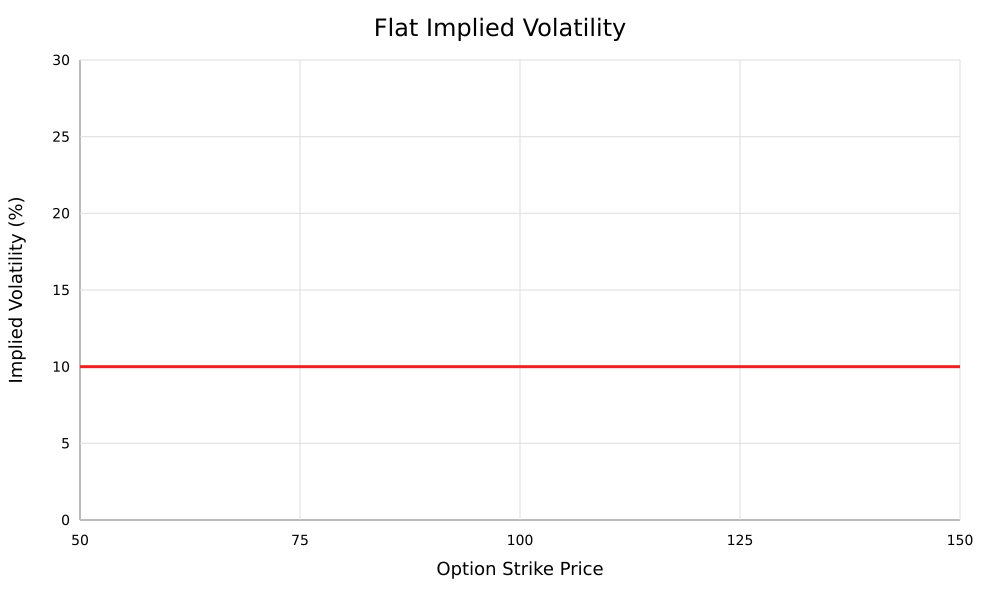
Illustrative flat implied-volatility curve across strikes; this is a schematic, not historical pre-1987 option-market data.

The Downside Volatility Smirk

The crash was an extreme left-tail event: in the historical S&P 500 series used below, the index fell 20.47% on 19 October 1987. It exposed the limits of treating volatility as constant through market stress.

Equity-index options display a persistent downside volatility smirk, with lower-strike puts generally trading at higher implied volatilities than at-the-money options. The literature links that shape to negative-jump risk, spot-volatility dynamics, and demand for downside protection. The chart below is an illustration of the shape, not a measured post-1987 option surface.

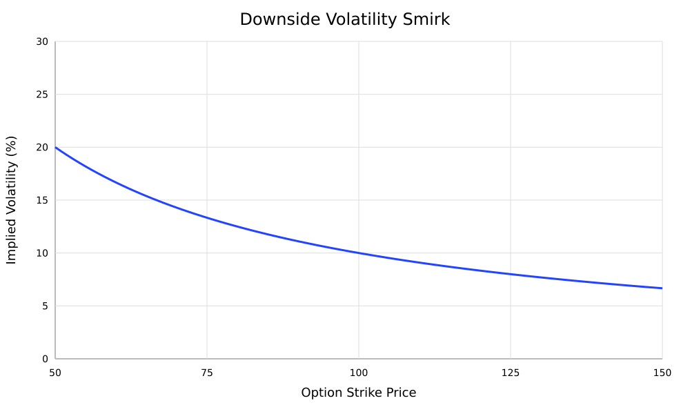
Illustrative downward-sloping implied-volatility curve across strikes; this is a schematic, not a measured post-1987 option surface.

---

The Mechanics of Skew and Vanna

Now that we know a little bit about the history of skew and the pricing of volatility by strike, we can examine why skew exists and the math behind it.

Why Does Skew Exist?

As we stated before, skew is the difference in implied volatility for OTM puts vs OTM calls. Therefore, option skew is:

Option Skew = The implied volatility (IV) of a specific delta out-of-the-money call option - the implied volatility (IV) of the same delta out-of-the-money put option

Positive skew implies that OTM calls have higher implied volatilities than OTM puts, and negative skew implies that OTM puts have higher implied volatilities than OTM calls.

Skew in the options chain reflects the empirical distribution of returns, market sentiment, and market demand for hedging against downside returns.

The first of those can be visualized below. The reference analysis uses 10,055 S&P 500 daily price returns from 3 January 1986 through 28 November 2025. The distribution has a longer downside tail: its most negative daily return is -20.47%, versus 11.58% on the upside.

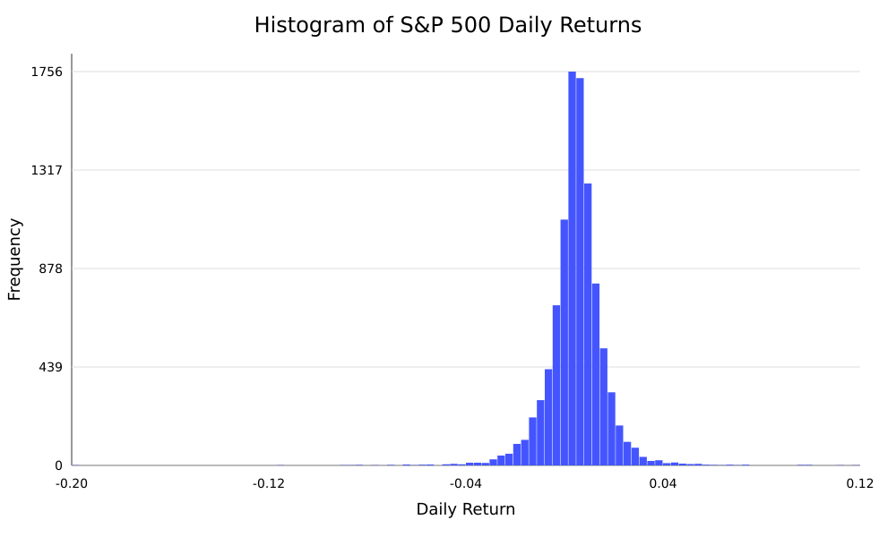
Historical histogram of 10,055 S&P 500 daily price returns from 3 January 1986 through 28 November 2025; the reference sample contains 23 gains above 5% and 27 losses below -5%.

This can also be seen with a simple calculation that shows the percent of historical daily moves above and below a return threshold. Under a symmetric distribution, the population probabilities above 5% and below -5% are equal, although a finite sample need not produce identical counts. In this sample:

Percentage of Daily Returns greater than 5.0%: 0.23%

Percentage of Daily Returns less than -5.0%: 0.27%

To give one more example of skew, but on a longer timeframe, we can do the same calculation for monthly returns given a specific threshold. I used 15% (positive and negative) for this example:

Percentage of Monthly Returns greater than 15.0%: 0.00%

Percentage of Monthly Returns less than -15.0%: 0.42%

These figures are consistent with downside asymmetry in this sample, although the 23-versus-27 daily count is small and the threshold choice is descriptive rather than a statistical test. In options, skew varies across markets and over time; this sets up the trading discussion in Part 2.

Skew also exists due to the market demand for hedges. Because of the return distribution and the net long position in equities by most investors and funds, there is a greater demand for OTM puts than OTM calls for downside protection. This pushes up the price and implied volatility of these OTM puts relative to the OTM calls.

This theoretical background is fascinating, but is there actual information value embedded in the skew? The academic literature suggests the answer is yes.