The Mechanics of Skew and Vanna: Part 1

[WITH CODE] Why is the Volatility Surface Skewed, and Can We Use It to Predict Returns?

Welcome back.

I have been working on this deep dive for a while, and I am excited to finally share it with you. Note: Due to the depth of this topic, I am splitting this analysis into two parts. Part 2 will be released tomorrow.

Today, we return to the mechanics of option pricing. Previously, I covered a post on an Introduction to Option Pricing, Greeks, and the Implied Volatility Surface and a post on how to construct the volatility surface.

In this post, we will start with a story (The Crash of 1987), move into the math of the volatility smile, and back it up with academic research and my own analysis. The code has been sent to your email.

Let’s get into it.

---

The Crash of 1987 (Black Monday)

On Monday, October 19, 1987, the Dow Jones Industrial Average (DJIA) fell 508 points, or 22.6%, marking the largest one-day percentage drop in the index’s history.

The decline was precipitated by macroeconomic factors, including concerns over high equity valuations, rising interest rates, and persistent U.S. trade and budget deficits. Specifically, on Wednesday, October 14, the House Committee on Ways and Means introduced a bill to reduce tax benefits for mergers and leveraged buyouts. Concurrently, the Commerce Department announced unexpectedly high trade deficit figures. In response, the dollar declined and interest rates rose. By Friday, October 16, the DJIA had already fallen approximately 5%.

Selling pressure accumulated over the weekend. Mutual funds received redemption requests exceeding their cash reserves, necessitating large equity sales at the Monday open. Additionally, “Portfolio Insurance” strategies (computerized algorithms designed to hedge portfolios by selling futures in declining markets) automatically triggered sell orders.

On Monday morning, a severe order imbalance occurred. Sell orders vastly outnumbered buy orders, preventing specialists from opening trading for 95 S&P 500 stocks and 11 DJIA components. However, the futures market opened on schedule. This created a price dislocation where futures traded at a steep discount to the spot market, transmitting further selling pressure back to the underlying stocks. By market close, the sell-off had overwhelmed the exchange’s systems and liquidity providers.

Before Black Monday: No Skew (Smirk) Priced in

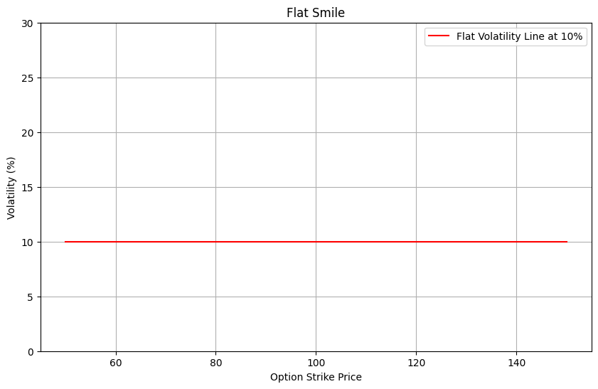
Prior to 1987, option pricing generally adhered to the assumptions of the Black-Scholes-Merton (BSM) model. A key assumption of BSM is that asset returns follow a log-normal distribution with constant volatility.

Because market participants largely accepted these assumptions, the Implied Volatility (IV) surface was relatively flat. As illustrated below, implied volatility was roughly constant across all strike prices; Out-of-the-Money (OTM) puts and OTM calls traded at similar implied volatilities. Traders did not price in a significant premium for extreme left-tail events (market crashes).

Hypothetical option smile (flat) for a stock that is currently trading at $100 (spot price = 100).

After Black Monday: Skew (Smirk) is Priced in

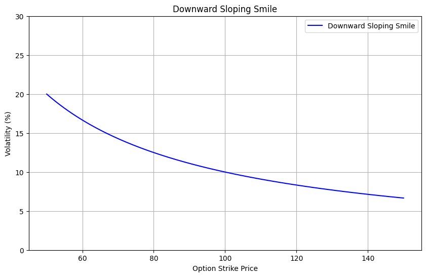
The 1987 crash demonstrated that market returns exhibit “fat tails” and are not normally distributed. The decline of over 20 standard deviations invalidated the assumption of constant volatility during stress events.

Following this event, the options market structurally repriced downside risk. As shown in the chart below, OTM put options (lower strikes) began trading at significantly higher implied volatilities than ATM or OTM call options. This persistent asymmetry is known as the volatility “skew” or “smirk.” It reflects the market’s expectation that correlation increases approaching 1.0 during sell-offs and that volatility is inversely correlated with spot prices.

Hypothetical option smile (downward sloping) for a stock that is currently trading at $100 (spot price = 100).

---

The Mechanics of Skew and Vanna

Now that we know a little bit about the history of skew and the pricing of volatility by strike, we can examine why skew exists and the math behind it.

Why Does Skew Exist?

As we stated before, skew is the difference in implied volatility for OTM puts vs OTM calls.¹ Therefore, option skew is:

Option Skew = The implied volatility (IV) of a specific delta out-of-the-money call option - the implied volatility (IV) of the same delta out-of-the-money put option

Positive skew implies that OTM calls have higher implied volatilities than OTM puts, and negative skew implies that OTM puts have higher implied volatilities than OTM calls.

Skew in the options chain reflects the empirical distribution of returns, market sentiment, and market demand for hedging against downside returns.

The first of those can be visualized below. I have created a chart that shows the daily returns of the S&P 500. While it is nearly impossible to see the actual observations in the histogram, the histogram depicts extreme negative moves, without extreme positive moves. This is evidenced by the fact that the range of moves to the downside are much greater than to the upside.

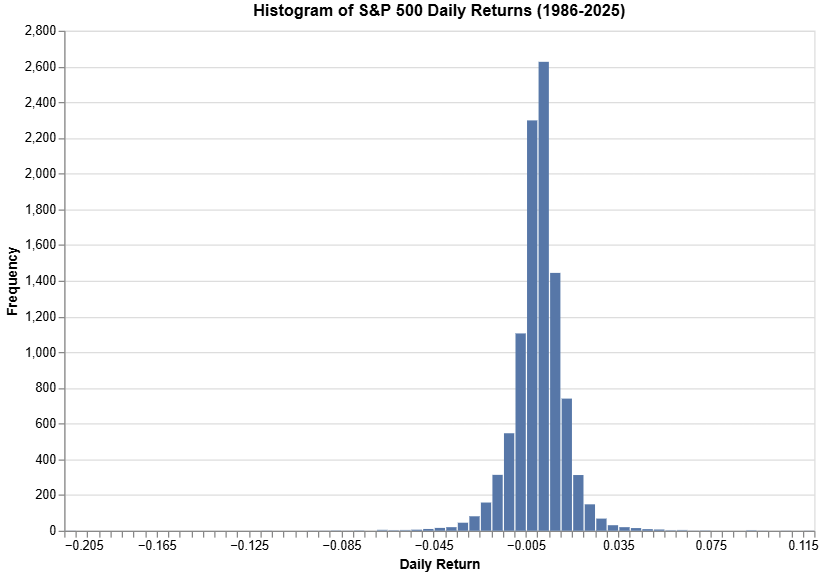
This can also be seen with a simple calculation that shows the percent of historical daily moves above and below a certain return threshold. In a normal, symmetric distribution, we would expect to see the same percent of the daily returns above 5% and below -5%. However, this is not the case:

Percentage of Daily Returns greater than 5.0%: 0.23%

Percentage of Daily Returns less than -5.0%: 0.27%

To give one more example of skew, but on a longer timeframe, we can do the same calculation for monthly returns given a specific threshold. I used 15% (positive and negative) for this example:

Percentage of Monthly Returns greater than 15.0%: 0.00%

Percentage of Monthly Returns less than -15.0%: 0.42%

There is a clear bias towards the downside in returns. This is skew empirically. Because of this, market participants also price in this skew, and price the skew to be higher in some markets than others, and also during some periods. This is the foundation for trading skew (which we will get into in the next section and next post).

Skew also exists due to the market demand for hedges. Because of the return distribution and the net long position in equities by most investors and funds, there is a greater demand for OTM puts than OTM calls for downside protection. This pushes up the price and implied volatility of these OTM puts relative to the OTM calls.

This theoretical background is fascinating, but is there actual information value embedded in the skew? The academic literature suggests the answer is yes.