

Hello and welcome back to another paid post!
Today we are looking at quarter-end funding pressure, and at whether it shows up in the rate everyone uses to measure it. Across the twenty-five ordinary quarter-ends in the SOFR record, the median spread between SOFR and the policy floor on the turn date is exactly zero basis points. Against ordinary month-ends the difference is 3.01 basis points with a p-value of 0.217. On the number that gets quoted, quarter-end is not a thing.
The same days, measured in the upper tail of the same distribution, look completely different. A quarter-end roughly doubles the dislocation there, and unlike the level result, it survives dropping September 2019. It scales with reserve scarcity: each percentage point lower on reserves as a share of bank assets raises it about 39%. The largest reading in the sample is not September 2019 either. It is June 2019, when the quoted rate ranked it sixth of twenty-five, unremarkable.
Let’s dive right in.
Introduction
The standard account of quarter-end in funding markets is that balance sheet constraints bind on reporting dates, dealers pull back from intermediating repo, and the overnight rate spikes. September 2019 is the canonical illustration. The mechanism is right. The question is where you can see it.
SOFR is a volume-weighted median. The New York Fed publishes it alongside the first, twenty-fifth, seventy-fifth, and ninety-ninth percentiles of the same day’s transactions, and the median is the only one of those numbers that gets quoted. On a normal day the choice does not matter much. On a turn date it matters enormously, because the marginal borrower who cannot find balance sheet is not transacting at the median. They are transacting in the tail, and the tail is a different series with different behavior.
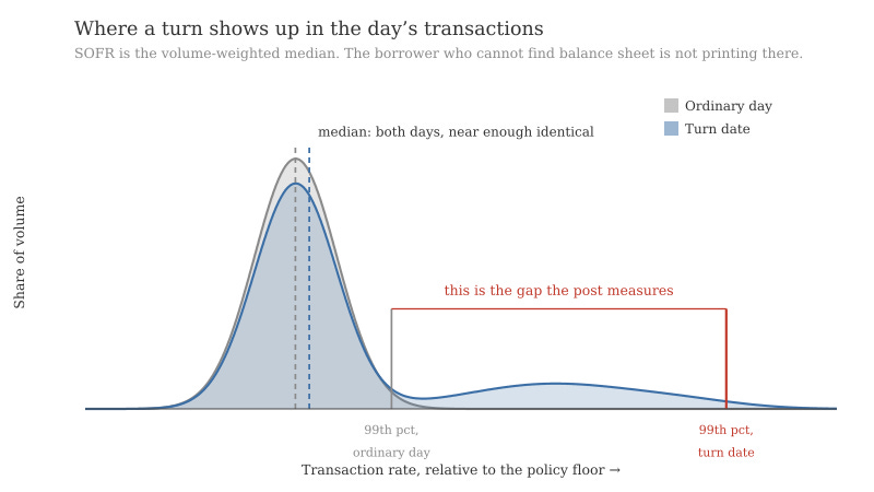
I want to be careful about what follows. This is not a trading strategy, and there is no instrument at the end of it. It is a measurement argument: a widely discussed phenomenon has been evaluated with the wrong statistic, and the right statistic tells a cleaner story about reserve scarcity than the wrong one does.
Data and Methodology
Everything here comes from two sources. The New York Fed’s markets API publishes SOFR, the tri-party and broad general collateral rates, and the effective fed funds rate, each with the full percentile distribution and daily volume, from 3 April 2018. FRED supplies interest on reserves, overnight reverse repo balances, reserve balances, the Treasury General Account, and total commercial bank assets. No API key is required for either.
Two construction choices drive most of what follows, and both are worth stating plainly.
Turn dates come from the observed rate calendar, not a calendar offset. Roughly a third of quarter-ends fall on a weekend and settle on the prior business day. Using MonthEnd or QuarterEnd offsets misaligns those, and since the effect is concentrated in a two or three day window, misalignment destroys it. I label every trading day by its position in the published SOFR series and define the turn window as one business day either side of the last observed trading day of the period.
The premium is measured relative to the ambient level, not to the policy floor. This one changed the whole analysis. When reserves are scarce, SOFR trades above the floor every day of the month, not only at turns. A model that regresses the raw turn-date spread on reserve scarcity will score well by predicting the ambient level while explaining nothing at all about the turn. So for each turn I compute the median spread over a reference window spanning twenty to five business days before and five to twenty business days after, and subtract it. What remains is the part specific to the turn date.
The correlation between the raw turn-date spread and the ambient level is 0.778. Most of what looks like quarter-end pressure in the unadjusted series is simply the funding regime you happened to be in that quarter.
The sample runs from April 2018 to August 2026 and contains twenty-five ordinary quarter-ends, sixty-seven ordinary month-ends, and eight year-ends. Year-ends are held out of every model and reported separately, because G-SIB scoring is a point-in-time measurement on 31 December and pooling them contaminates both groups. Twenty-five observations is a small sample, and I will come back to what that rules out.
Predictors are read five business days before each turn, using only vintages published by then. Reserve balances and bank assets are weekly for the week ending Wednesday and appear in the H.4.1 the following Thursday, so the code enforces that Wednesday W is not available until W+1 rather than merging on nearest date. The reserve ratio is reserve balances as a percentage of total commercial bank assets, which ranges from 7.99% at the September 2019 blowup to 19.26% at the peak of the abundant-reserve period, and sits at 11.48% today (the most recent reading).
Results
Here is the level measure, and it is a null result.
The turn-specific excess averages 7.58 basis points at quarter-ends and 4.57 at ordinary month-ends. The difference is 3.01 basis points with a Welch p-value of 0.217 and a Mann-Whitney p-value of 0.177. Neither test comes close to conventional significance. On the raw unadjusted spread the picture is worse: the quarter-end mean is 2.16 basis points, the median is exactly zero, and twelve of the twenty-five quarter-ends printed a negative spread, with SOFR below the floor.
Pooling quarter-ends and month-ends into a single regression with a quarter-end dummy, controlling for the reserve ratio and overnight reverse repo balances, gives a dummy of +3.33 basis points at p=0.034. That looks like a result until you remove September 2019, at which point it falls to +1.86 and p=0.163.
Fitting the excess on reserve scarcity gives an in-sample R-squared of 0.346 and a leave-one-out R-squared of 0.091. Removing September 2019 takes the reserve coefficient from −2.02 to −0.91 and its p-value from 0.014 to 0.136. Restricting to 2020 onward, which is the regime anyone would actually care about, the leave-one-out R-squared goes negative, at −0.195. Worse than predicting the sample average.
September 2019 has a Cook’s distance of 1.011 and a studentized residual of 4.76. Those are not the numbers of an influential observation. They are the numbers of a different data-generating process that happens to be sitting in the sample.
The level measure says quarter-ends are not special, the relationship with reserves is one repo crisis, and nothing here supports a forecast. But the percentile columns say otherwise.