Origins of Bond Convexity and Convexity Bias

[WITH CODE] An analysis of the price-yield relationship, the Taylor Series expansion, and the structural convexity bias between futures and swaps

Hello!

Welcome back to another market investigation. Since you all loved the last series where we explained market structure with the underlying math and investigated inefficiencies, I wanted to stay on the same theme.

Today, we will discuss the price-yield relationship in bonds, how Taylor Series explain the origins of duration and convexity, convexity bias, and how to trade convexity bias.

Additionally, there are some fascinating research papers on this topic that we will explore.

Let’s get into it.

---

Bond Price-Yield Relationship

This post will start off simple, but gradually get more complex. Stay with me for the simple introduction; it will make sense later in the post.

Let’s say we have a stock XYZ that is priced at $100, and we buy one share of the stock. If the stock appreciates by 1% the next day, the new price is $101, and our P&L is $1. Simple.

Now, let’s say we own a zero-coupon bond with 10 years to maturity. Currently the bond yields 5%. If interest rates fall by 10 basis points (new yield is 4.90%), what is the new price of the bond? What is our P&L?

As many of you know, bond movements are not quoted in percent price changes (like stocks), but in yield changes (basis points). Crucially, a 1% change in yield does not equal a 1% change in price. Because the yield is in the denominator, the relationship is non-linear.

Rather, bonds are priced by summing the expected future cash flows of the bond, and then discounting them to the present value. The equation is displayed below.

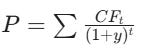
Because (1+y) is in the denominator, the function curves inward toward the origin. A depiction of this relationship is below:

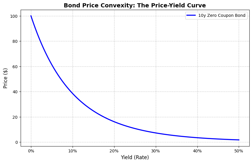
Not only is there a difference in your P&L for a given 1bp move depending on what the current yield is (duration), but your gain from a 1bp fall will be greater than your loss from a 1bp rise (assuming you are long the bond).

The mathematical reasoning on why a bond has a convex relationship between price and yield is due to the price formula above, and what the derivative of the formula looks like.

Let’s say we have a linear function, where:

k is a constant

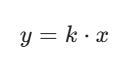
When you take the derivative (find the rate of change), you apply the power rule: multiply by the exponent (1) and subtract 1 from the exponent:

Therefore, the x disappears, and your “rate of change” is simply k. This relates to equities, as your P&L is (and always will be) your exposure to the stock (times the return of the stock).

However, for a bond, it is different. To see why this happens mathematically, let's simplify the complex bond formula down to its most basic structural form: an inverse function:

k is a constant

When you take the derivative here, the math changes because of that negative exponent.

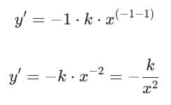
The x stays in the equation. If you take another derivative, the x will be pushed to the cubed power. This looks similar to that of the bond price equation, which is why there is convexity in interest rates.

Because the rate of change is constantly changing based on where you are, the line must bend (positive convexity).

To summarize:

In a linear model, the variable x disappears from the risk equation, and your risk (duration) is constant.

In a convex model, the variable x remains in the risk equation (squared!), and your risk changes every time the market moves. That surviving x is the source of convexity.

This leads us into our next section.

---

Taylor Series Expansion

Now that we understand the “why” (the inverse relationship between price and yield), let’s look at the “how.”

To mathematically quantify this relationship, we use a Taylor Series expansion (which we used a few posts ago). In calculus, a Taylor Series allows us to approximate the value of a complex function at a new point based on its derivatives at a known point.

In our case, we want to estimate the new Price of a bond if yields change by a small amount. To do this, we treat the bond pricing formula from the previous section as a function of yield, denoted as P(y).

If we only used the first derivative (Duration), we would be assuming the relationship is a straight line. As we proved in the previous section, it is not. To get a more accurate price, we must add the second derivative (Convexity) to the equation.

Here is the Taylor Series expansion for a bond price:

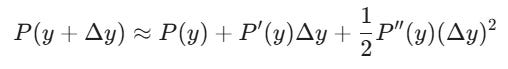
This formula might look dense, but we can translate it into the trading terms we use every day. P’(y) is the first derivative, which is duration, and P’’(y) is the second derivative, which is convexity.

When we divide both sides by the Price (P) to get the percentage return, the equation simplifies into the standard risk formula used by portfolio managers:

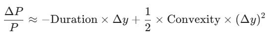
This equation reveals the mathematical "magic" of convexity. Look closely at the second term:

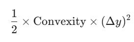
Because (Δy) is squared, the result is always positive, regardless of whether rates go up (+Δy) or down (−Δy).

• If rates sell off (+100bps), the Duration term hurts you, but the Convexity term adds positive value, cushioning the loss.

• If rates rally (-100bps), the Duration term helps you, and the Convexity term adds even more positive value, boosting the gain.

Here’s a visualization of the price-yield relationship along with the duration and duration + convexity approximations from the Taylor Series.

The chart above visualizes the Taylor Series in action. The Red Line (Duration) assumes a straight path, which is accurate for tiny moves, but dangerous for large ones. The Green Curve (Convexity) adds the squared term, bending the approximation to match reality almost perfectly. To be even more accurate, one would need to get the 4th and 5th terms for the Taylor Series, but that is a conversation for another day.

While Duration is a linear bet on direction, Convexity is a structural bet on volatility. The more yields move (the larger the Δy), the more valuable that squared term becomes.

This naturally leads to a conflict in the market. If one instrument (like a Bond or Swap) has this “positive convexity” term, and another instrument (like a Future) does not, they cannot trade at the same yield. The market must price in a premium for that variance.

This phenomenon is known as the Convexity Bias.

---

Convexity Bias

This natural difference in geometry (the red line vs. the green curve) leads to a structural inefficiency in the market known as Convexity Bias.

As we established in the previous section, convexity is valuable. It acts as a natural “shock absorber” for your portfolio, cushioning losses when you are wrong and accelerating gains when you are right. But in efficient markets, there is no such thing as a free lunch. If an asset has a mathematical advantage, you have to pay for it.

This brings us to the structural conflict between Futures and Swaps. While both instruments allow you to bet on interest rates, their payoff structures are fundamentally different. Futures (like SOFR or Eurodollar futures) are settled daily. Because your gains or losses are credited to your account every single day, the compounding effect is removed, effectively making the instrument linear (zero convexity).

Swaps and Forwards, however, are settled at maturity. Because the cash flows are discounted back from a future date, they retain the non-linear math we discussed above. They are convex.

If you are Long a Swap, you own the “Green Curve” from our chart above. If you are Long a Future, you own the “Red Line.” Since the Green Curve mathematically outperforms the Red Line in a volatile environment, the Swap is the superior instrument. Therefore, the market forces a premium on it. The Swap Price must be higher than the Futures Price. And since Price and Yield are inverse, the Swap Rate must be lower than the Futures Rate.

This yield differential is the Convexity Bias.

We can quantify exactly how large this wedge should be. According to the seminal research by Burghardt & Hoskins, the relationship is defined by volatility:

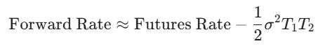
Look at the minus sign in the equation. The Forward Rate (Swap) trades below the Futures Rate. The size of that discount depends entirely on the variance. In calm markets, the bias is small, and Futures and Swaps trade near parity. In volatile markets, the bias is large. The “value” of that convexity increases, forcing the Swap rate significantly lower than the Futures rate.

This effectively turns the spread between Futures and Swaps into a proxy for volatility itself. And if it’s a proxy for volatility, that means we can trade it.