Modeling Prediction Markets As Exotic Options Part 2

[WITH CODE] Building a dashboard and fair value model for temperature derivatives

Hello!

Welcome back to the second post in this series. Last week, we covered the structure of digital and digital range options and their associated greeks.

Today, we’ll dive deeper into modeling these digital range options with historical data from a Kalshi Market. I have sent the code and data to your email.

Let’s get into it.

---

The 5-Strike Model and Implied Spot

By looking at the different between contracts on Kalshi, we can effectively back out the market’s expected volatility. If the price for a narrow range like 90 to 91°F is very high, the market is pricing in low volatility, and high certainty that the true temperature will be in this bucket.

If that price drops while other ranges like >93°F rise, the market is pricing in a fatter tail event. Pin risk remains the primary danger in these markets. If the temperature is hovering exactly at 90.0°F as the market expires, your position value will oscillate violently between $0 and $1. This causes your Gamma to approach infinity, making the position nearly impossible to manage or hedge as you approach the cliff (but you can’t delta hedge in many prediction markets, as you can’t trade the underlying temperature!).

The mathematical foundation of this model rests on the observation that Kalshi’s exhaustive probability buckets implicitly define a cumulative distribution function. While these between contracts are displayed as a one degree difference, such as 78 to 79°F, they actually represent two degree differences in reality. This is because each between contract is bounded by the half degree midpoints between adjacent buckets. For example, a contract labeled 78 to 79°F is effectively a bet that the temperature lands between 77.5 and 79.5. By summing these bucket probabilities from the bottom up, we can construct five synthetic digital call prices at the true cliff boundaries of 75.5, 77.5, 79.5, 81.5, and 83.5.

We avoid the classical log-normal Black-Scholes framework because temperature does not grow multiplicatively like a stock price. Instead, we utilize an additive normal distribution model where the settlement temperature is modeled with a market-implied mean and a market-implied standard deviation in degrees Fahrenheit.

This approach is appropriate because using % moves do not make sense, as a forecast of 80°F does not necessarily mean greater degree moves than a 50°F forecast. Applying a log-normal model to weather would create artificial skews that do not exist in physical reality.

Rather than manually inputting a temperature forecast from an external source, the dashboard solves for the market’s implied mean directly from the bucket prices.

We compute a discrete mean as a probability-weighted average of bucket midpoints to provide a fast and intuitive estimate of the consensus. However, the model primarily relies on a continuous mean derived by fitting a normal distribution to our five synthetic strike data points using the Nelder-Mead optimization algorithm.

This fitted mean is significantly more robust than a simple discrete average because it utilizes the full distributional shape and naturally handles inconsistencies where tail contracts might be priced poorly relative to the center of the book. This continuous mean serves as our spot price for every subsequent pricing and Greek calculation.

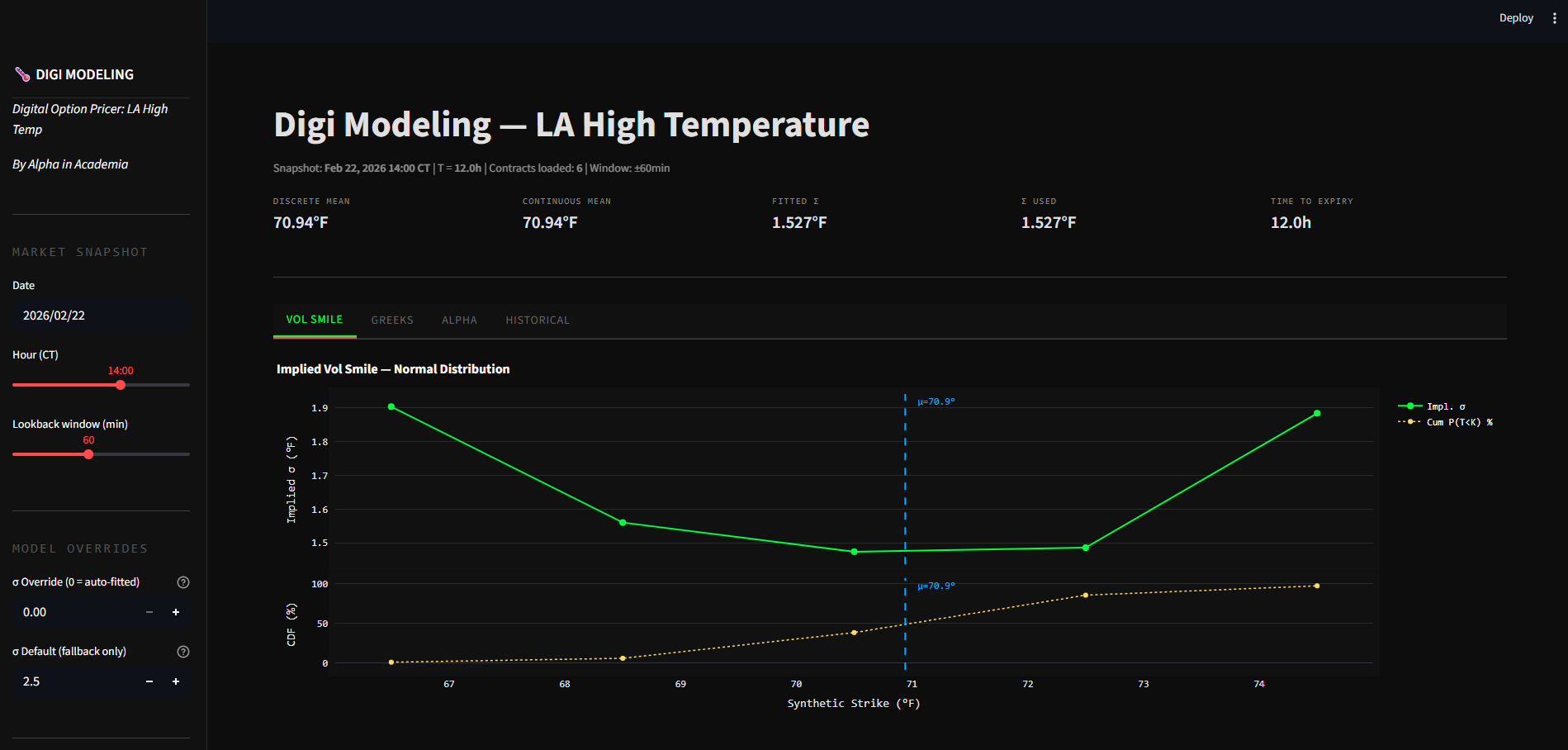
Below, I’ll walk through the dashboard (which you all have access to), and I’ll show how we can use our own implied vol calculations to determine how contracts are mispriced.