
LETFs: Structural Arbitrage & The Mathematics of Decay
Why 3x Leverage is Mathematically Flawed (and the 2.0+ Sharpe System That Exploits It)

Reviewed and updated 20 July 2026
Hello!
Welcome back. Today, we will be looking further into a topic that I wrote about in the past: volatility decay. Also known as beta slippage or volatility drag, this is a neat concept that helps us understand the structure of the market.
In my opinion, it is crucial for everyone to understand this, as this concept (or similar concepts) appear(s) in all markets.
At the end, I will share a recent working paper whose strongest U.S. bull-side specification reports a Sharpe ratio of 2.12. A research companion for the compounding and leverage examples is included below.
Let’s get into it.
Recap
In my first post on this topic, LETFs: Volatility Decay & Optimal Leverage, I explained how LETFs utilize derivatives and daily rebalancing to amplify daily index returns. We broke down the mechanics of “volatility decay,” demonstrating mathematically how choppy markets erode capital and why this drag accelerates with higher leverage.
Despite common warnings against holding LETFs long-term, we introduced research on “Optimal Leverage,” which suggested an optimal leverage (that was not 1x!) for historical US markets.
In my second post on this topic, LETFs: Dual Strategies for Smarter Leverage, I examined two leveraged ETF strategies. The first strategy used LETFs to construct a leveraged variation of the traditional 60/40 portfolio. While this portfolio delivered exceptional gains from 2009 through 2021 aided by negative stock-bond correlations, the strategy suffered losses in 2022 when rising interest rates caused both asset classes to decline simultaneously.
The second strategy in the post amplified outperformance relative to the benchmark (S&P 500) by capitalizing on lower prices during drawdowns.
All About Returns
Today, we are going to stick with analysis in the U.S. equity markets. A common modeling assumption is that continuously compounded returns are normally distributed; under its standard assumptions, Black–Scholes implies lognormal prices. Real returns exhibit skewness, fat tails, jumps, and changing volatility, but a normal-return approximation is useful for the simplified derivation below.
In finance, your wealth at time T (WT) is not the sum of your daily returns; it is the product of your daily growth factors. If xi is your return on day i (e.g., +0.05 or -0.02):
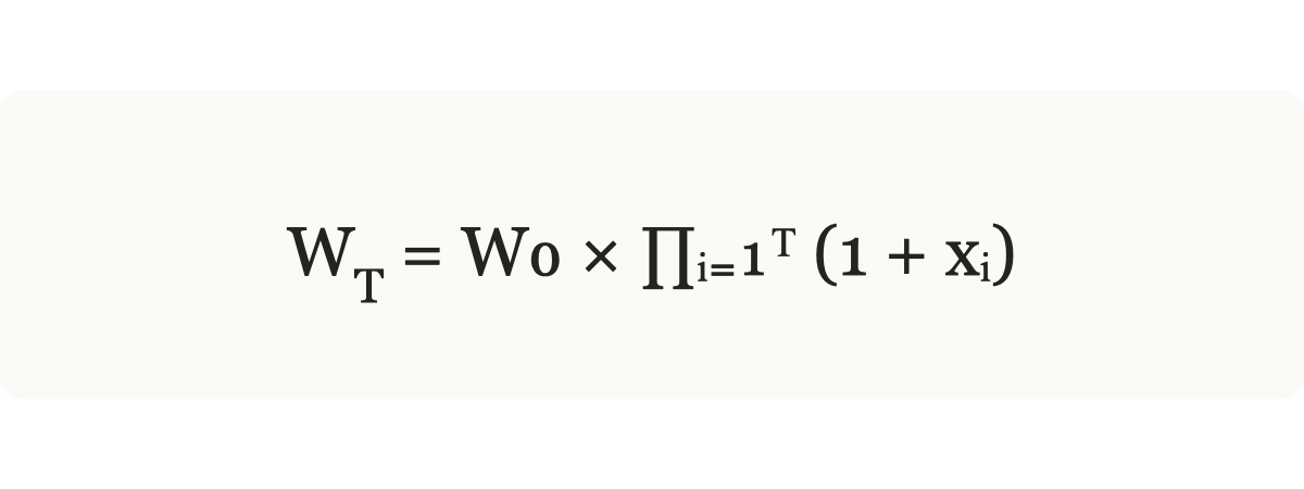
This is, in essence, compounding, We want to find the single rate G (Geometric Growth) that represents this messy path:
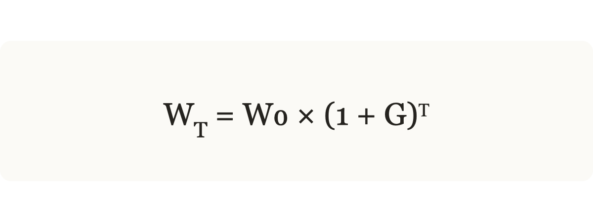
We can then take the natural logarithm (ln) of both sides:
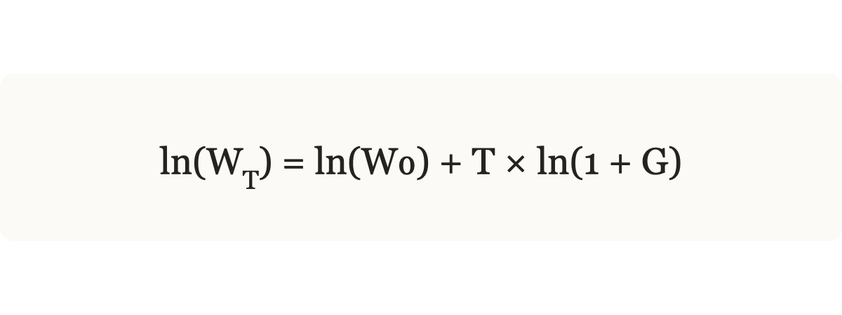
Because ln(a * b) = ln(a) + ln(b), the product turns into a sum:
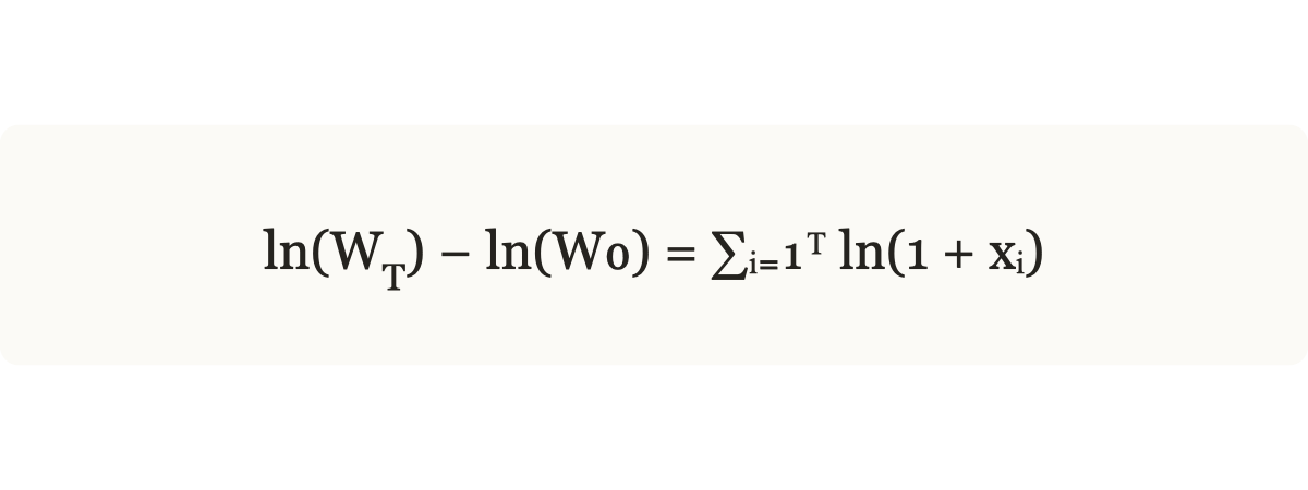
If we ignore the starting wealth, we are simply left with the summation of the log returns (ln(1+x)).
But, why do we use ln(1+x)?
If you have a discrete return x (like +10%), the ln(1+x) calculates the continuously compounded return required to achieve that same result. For example, if a stock appreciated 10%, the continuously compounded return would be 9.53%, as ln(1.10) = 9.53%. Therefore, ln(1+x) transforms the discrete return into its continuous equivalent.
This is helpful as wealth accumulation is a multiplicative process, but statistical tools (like mean and variance) work best on additive processes. The logarithm is the tool that converts the former into the latter, and this makes them mathematically elegant for computers and researchers.
Additionally, log returns make multiplicative moves additive. For example, if stock XYZ starts at $100, rises 10% on day 1, and falls 10% on day 2, it ends at $99. The two log returns are approximately +9.53% and −10.54%, respectively, and sum to ln(0.99), or about −1.01%.
Equal and opposite log returns do return the underlying to its starting value. In simple-return space, a 10% gain requires a 9.09% loss to reverse it; equal +10% and −10% simple returns do not cancel.
Taylor Series
In this part, I will give a refresher on Taylor series and how it connects to the concept of vol decay.
A Taylor Series approximates any complex, curved function (like a logarithm or sine wave) using a sum of simple polynomial terms (like x2, x3, x4).
The general formula for approximating a function f(x) near a point a is:
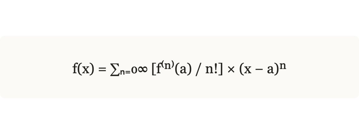
As we saw above, we care about Geometric Growth, which is governed by logarithms. Therefore, we can use a Taylor series to approximate the the function ln(1+x). I won’t do all the math out (as it is difficult in Substack), but this is the final approximation to two derivatives.
We approximate at 0 as daily returns are close to 0 and you want to approximate as close to the majority of your data points as possible (once again, assuming a roughly normal distribution of returns). A return of 0% is roughly the mean return on any given day for the S&P 500.
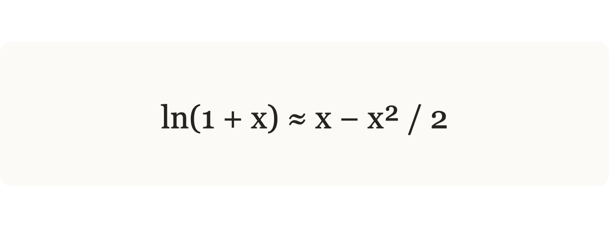
The −x²/2 term is the second-order curvature adjustment. Averaging the approximation gives expected log growth of roughly the arithmetic mean minus half the second moment. Because E[x²] = Var(x) + E[x]², the familiar mean-minus-half-variance expression also treats the squared mean as negligible at the chosen interval.
In formal finance terms, volatility decay creates a divergence between the Arithmetic Mean (simple average) and the Geometric Mean (compounded growth).
The approximation formula for this relationship is:
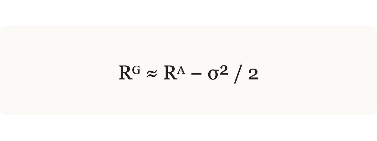
This is the familiar approximation linking arithmetic and geometric averages. Holding the arithmetic mean fixed, higher variance lowers approximate log growth. It is an approximation for small interval returns, not an exact identity for every return distribution.
Deriving the Levered Formula
Now, let’s connect this all to LETFs. Simplistically, LETFs target a multiple of each underlying daily return. As you all know, I do not view volatility decay as some evil spirit that automatically justifies avoiding LETFs; compounding affects every volatile return stream.
Instead of trying to avoid volatility decay, we can ask what leverage (0.5x, 1x, 2x, 5x?) maximizes the model’s expected log growth. In this approximation, the variance penalty rises with leverage squared—not exponentially.
The paper I discussed in the earlier post estimated optimal leverage through backtests, but there is also an elegant mathematical approximation that helps explain its findings.
In this mathematical optimization, we want to maximize the Geometric Growth Rate, not the Arithmetic Mean. However, before we solve for optimal leverage, we need to derive the levered formula.
The return of your levered portfolio (RL) is the risk-free rate plus the leveraged excess return:
RL = r + f (Rm - r)
Rm is the market return, r is the risk-free rate, and f is the leverage. To find the Geometric Growth (g), we take the expected value (E) of the log return:
g = E [ ln(1 + RL) ]
Then, taking our Taylor approximation from above (x-(x2/2)), we can substitute:
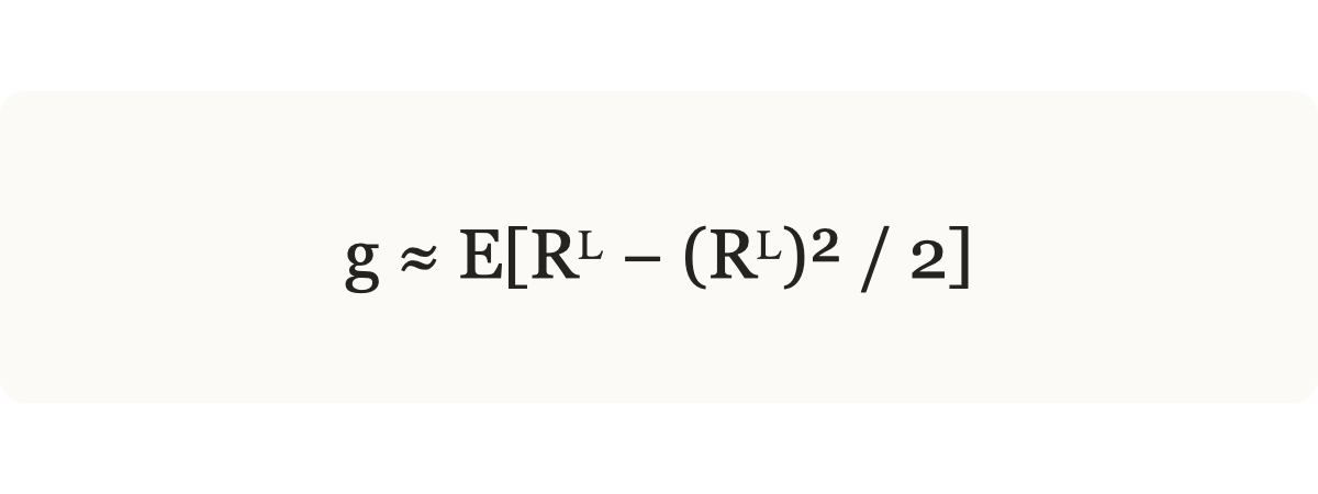
And then simplify:
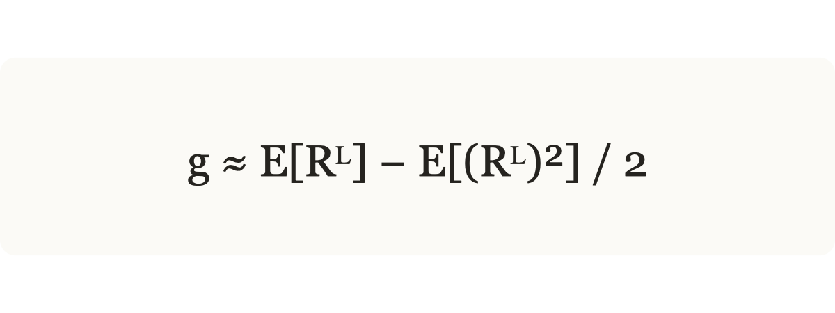
1) The linear term is simply expected return:
E[RL] = r + f*(µ- r)
2) Now, onto the squared term (E[RL2]). We need to square the levered return formula (from above). For small time intervals, the risk-free rate part becomes negligible when squared compared to the volatility, so we approximate RL = f * Rm for the variance term.
RL2 ~= Rm2 * f2
In statistics, E[X²] = Var(X) + E[X]². For short intervals, the squared mean is often small relative to the variance, so this derivation approximates E[X²] by σ².
E[RL2] ~= σ2 * f2
3) Now, we can substitute the prior steps into the geometric equation.
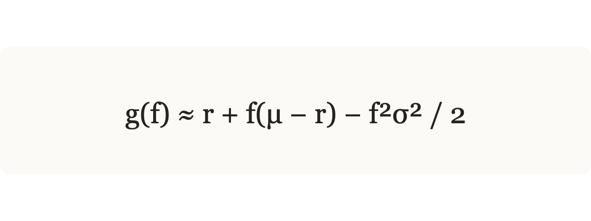
And, there we go. That is the geometric return for the levered portfolio. It took a bit to get here, but now the fun part comes. In the next section, we will find the optimal leverage formula, and showcase the strategy.
Optimal Leverage
To find the optimal leverage, we take the derivative of the geometric growth with respect to leverage (f) and set it to zero:
Keep reading with a 7-day free trial
Subscribe to Alpha in Academia to keep reading this post and get 7 days of free access to the full post archives.