Convexity of Vega (Volga) Part 1

How your vega exposure changes as implied volatility changes, backed with academic papers

Reviewed and updated 24 July 2026

Hello!

Welcome to the start of a new two-part series. Two and a half months ago, I explained the concept of skew and vanna, and the anomalous findings in academic papers (Part 1 and Part 2). Today, we are going to investigate Volga (not the river in Europe) and kurtosis.

Volga (also known as Vomma) is a second order option Greek (like gamma and vanna) and is very important on institutional trading desks but not understood by the average retail trader.

Let’s get into it.

---

The Fall of LTCM

In 1998, Long-Term Capital Management (LTCM) nearly collapsed after a highly leveraged portfolio of convergence trades moved sharply against it. Myron Scholes and Robert Merton were among the fund’s partners, but the failure cannot be reduced to one Black-Scholes assumption: leverage, crowded positions, liquidity, funding pressure, and model risk all mattered.

The fund sought small price discrepancies between related securities, including positions in on-the-run and off-the-run Treasuries. Because the expected spreads were small, LTCM used substantial leverage. That made losses and collateral demands severe when spreads widened together instead of converging.

The first signs of trouble appeared in early 1998 as losses reduced the fund’s capital. Its risk estimates were poorly equipped for a market in which correlations changed, liquidity disappeared, and many investors tried to exit similar positions at once.

Russia’s August 1998 default intensified a global flight to safety. Positions that looked diversified under ordinary conditions became exposed to the same liquidity shock, and the fund’s leverage magnified the result. Describing this as a precise “10-sigma” event gives a false sense of accuracy because that number depends entirely on the model and calibration.

LTCM lost about $4.6 billion in 1998. The Federal Reserve Bank of New York helped coordinate a $3.625 billion private recapitalization by the fund’s major creditors; this was not a taxpayer cash injection. The episode remains a useful warning about leverage, liquidity, crowded trades, and treating thin-tailed model outputs as dependable descriptions of stressed markets.

Extreme market moves occur more often than a fixed normal model would imply. That is the starting point for today’s discussion of kurtosis and option prices.

---

Kurtosis

In the Black-Scholes-Merton model, the underlying follows a geometric Brownian motion, so continuously compounded returns over a fixed horizon are normally distributed and prices are lognormally distributed. Real return distributions can display skew and excess kurtosis that this baseline model does not capture.

LTCM shows why model assumptions must be considered alongside leverage, liquidity, and the possibility that market relationships change in a crisis.

I discussed skew in the earlier series; the focus here is kurtosis and fat tails. Headlines sometimes label market moves as “six-sigma” or “22-sigma” events, but those labels are not model-free facts. They depend on the return horizon, volatility estimate, lookback window, and distributional assumptions. The reliable point is simpler: a fixed Gaussian model can assign vanishing probabilities to moves that financial markets nevertheless experience.

A distribution with kurtosis above 3—or positive excess kurtosis—is called leptokurtic. The normal distribution has kurtosis 3 and excess kurtosis 0. The illustration below compares a normal density with a variance-standardized fat-tailed Student t density.

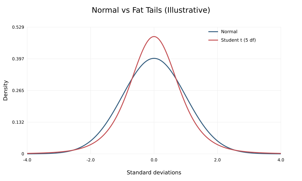
Illustrative normal and variance-standardized Student t densities. The Student t example places more probability in the far tails.

The defining feature here is the greater probability in the far tails, not the exact height of the center. Different distributions can have the same kurtosis while differing elsewhere in their shape.

Under the Black-Scholes-Merton assumptions, implied volatility would be constant across strikes for options with the same maturity. A 15% implied-volatility quote would therefore be the same for an out-of-the-money put and an at-the-money option, although their dollar premiums would still differ.

Actual option markets do not produce a flat surface. Supply and demand, crash risk, stochastic volatility, and jumps can all contribute to higher implied volatilities away from the center. That strike dependence produces a smile or, in many equity markets, a downside smirk.

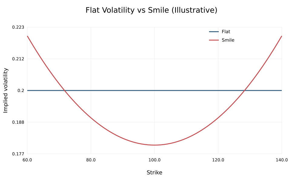
Illustrative flat-volatility benchmark and smile. This is a teaching curve, not a fitted market surface.

The curvature is one way the market departs from the constant-volatility benchmark. A steeper smile may reflect risk-neutral tail probabilities and tail-risk compensation, but it is not a pure or direct measurement of kurtosis alone.

This brings us to Volga and to research on the relationship between tail risk, option prices, and subsequent returns.