
Beyond the Expected Value
[WITH CODE] The Full Probability Distribution of a European Call Option at Expiry: Derivation, backtest, and what it actually tells you about your position.

Hello and welcome back to another paid post!
Today we will take a look at how the Boltzmann Framework (a 150-year-old equation originally designed to describe gas particles) gives us something Black-Scholes never did: the full probability distribution of what your option is worth at expiry, not just its expected value.
Let’s dive right in.
What Black-Scholes Is and Is Not
The Black-Scholes formula is one of the most used equations in all of finance. But it is worth being precise about what it actually gives you, because there is a common confusion about this.
Black-Scholes gives you the expected value of an option’s payoff under a specific probability model. That is it. One number. It tells you what the option is worth on average, in expectation, discounted back to today.
For pricing, that is exactly what you need. When you buy or sell an option, you want to know its fair value. The expected payoff, discounted, is that value.
But for risk management, one number is not enough. If you hold a call option on a stock that is currently trading just below the strike with two months to expiry, what you actually want to know is:
• What is the probability this expires worthless?
• If it does pay off, what range of outcomes should I plan for?
• How does that probability change as the stock moves day by day?
Black-Scholes does not answer these questions. It gives you the mean of a distribution it never shows you. What follows is a derivation of that full distribution, a backtest of how well it calibrates in practice, and an honest assessment of where it holds and where it breaks down.
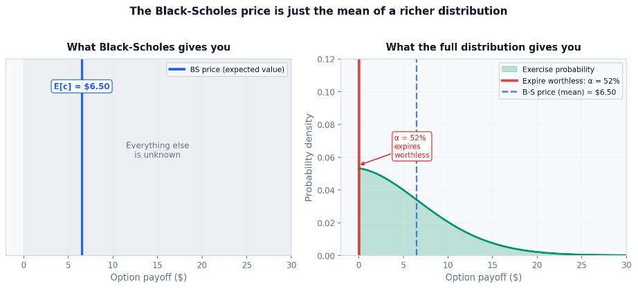
Figure 1: Black-Scholes gives you a single expected value. The full distribution tells you the probability of expiring worthless and the range of possible payoffs if it does not.
Deriving the Distribution
We model the log-price of the underlying stock as:
xₙ | x₀ ~ N( x₀ + (N–n)μ, (N–n)σ² )
where x = log(S) is the log stock price, μ is the daily drift, σ is the daily volatility, and N–n is the number of days remaining to expiry.
This is the assumption that underlies the Black-Scholes model — geometric Brownian motion. We will test this assumption rigorously later. For now, we work within it.
A European call with strike k pays at expiry:
c = (Sₙ – k)⁺ = [exp(xₙ) – k] · H[exp(xₙ) – k]
where H is the Heaviside step function (1 if the argument is positive, 0 otherwise). At any date before expiry, c is itself a random variable — its value is unknown. What does its probability distribution look like?
The key formula
Using a generalized change-of-variables formula based on the Dirac delta function, we can write the probability density function (PDF) of the payoff c as:
Ψ(c, N) = α · δ(c) + (1–α) · γ(c, N)
This is the central result. The distribution splits into exactly two parts.
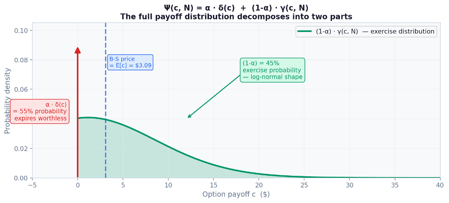
Figure 2: The full payoff distribution Ψ decomposes into a spike at zero (the option expires worthless with probability α) and a continuous distribution γ(c,N) for the payoff if it does exercise. The Black-Scholes price is the expected value of this entire distribution.
Alpha: the default probability
The first component is a spike at c = 0. This represents the probability that the option expires worthless (the stock ends below the strike and you lose the premium). The size of this spike is:
α = ½ · erfc ( (x₀ + (N–n)μ – log k) / (σ√(2(N–n))) )
In other terms: α is determined by how far the expected future log-price is from the log-strike, scaled by the uncertainty in that log-price. When the stock is deep below the strike, α is close to 1. When it is well above, α is close to 0. You can compute it daily as the stock moves.
Think of α like a probability of rain. When the forecast is for a 70% chance of rain, it doesn’t mean it will definitely rain. It means that in 100 similar situations, it rains 70 times. Alpha works the same way: α = 0.72 means that in similar market conditions with similar time to expiry and similar distance from the strike, the option expires worthless 72% of the time.
Gamma: the exercise-conditional distribution
The second component is γ(c, N), which is a log-normal distribution describing what the payoff looks like conditional on the option actually being exercised. This is a shifted log-normal in (k + c):
γ(c, N) ∝ (1/(k+c)) · exp(–[log(k+c) – (N–n)μ – x₀]² / (2(N–n)σ²))
The key properties of γ: it is right-skewed (large payoffs are rarer but possible), it spreads out with longer time to expiry, and it shifts right as the stock price rises above the strike. The 1/(k+c) factor means payoff density decays faster than the log-price density, meaning the deep in-the-money gains are less probable than the underlying stock movement alone would suggest.
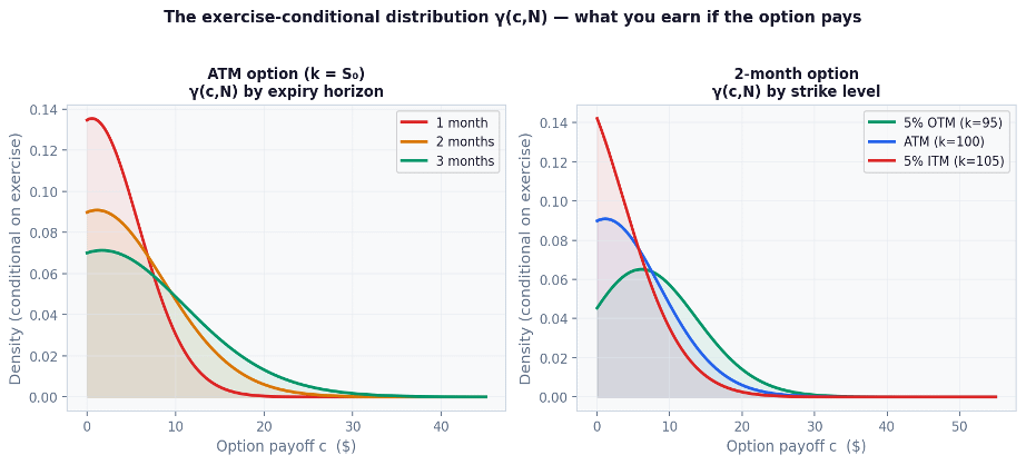
Figure 3: Left — γ(c,N) for an at-the-money option at three horizons. Longer expiry spreads the distribution and shifts the mode right. Right — γ(c,N) for three strike levels at a fixed 2-month horizon. An ITM option has a distribution shifted further right.
Recovering Black-Scholes as a special case
A useful sanity check: if you take the expected value of Ψ(c, N) over all c ≥ 0, you recover exactly the Black-Scholes price integral. Numerically, the difference is less than $0.0001 for all tested horizons.
This confirms that Black-Scholes and the full distribution are consistent. Black-Scholes is not wrong, but it is simply incomplete. It gives you the mean of Ψ without telling you the shape.
Tracking Alpha Over a Position's Life
One of the most practical applications of α is as a live risk monitor. You re-estimate μ and σ from recent price history and recompute α each day. As the stock rises above the strike, α falls. As it falls below, α rises. As expiry approaches, α converges to either 0 or 1 depending on where the stock is relative to the strike.
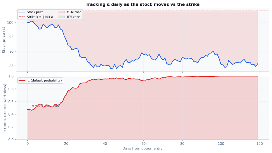
Figure 4: Top — a simulated stock path relative to the strike k = $104. Bottom — the corresponding α tracked daily. When the stock falls into the OTM zone, α rises. When it climbs above the strike, α drops. Near expiry, α converges rapidly.
This is more information than a simple delta or moneyness metric. Delta is a sensitivity measure (how much the option price moves per dollar of stock movement). Alpha is a probability (what the market-implied chance is that you walk away with nothing). They measure different things.
Practical use case
If α rises above 0.80 and you hold a long call position, the distribution is telling you there is an 80% chance of expiring worthless. That may or may not be actionable depending on your thesis, but it is a clean, calibrated number to use in position-sizing and stop-loss decisions.
Does It Work? A Backtest
The setup
We run a systematic backtest to answer the most important question about any risk metric: does the predicted probability match the realized frequency?
We simulate 3,500 trading days of price data (~14 years), construct synthetic call options at five different strike levels and three expiry horizons on every entry date, compute α using rolling estimates of μ and σ, then check how often options in each predicted-α bucket actually expire worthless. This produces roughly 47,800 option observations.
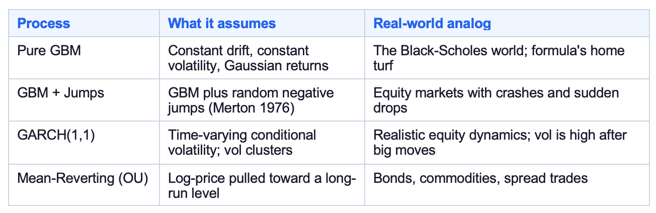
We run this across four different price-generating processes, each representing a different assumption about how markets behave:
The calibration result under GBM
The reliability diagram below is the key output. The x-axis is the predicted α; the y-axis is the fraction of options in that bucket that actually expired worthless. A perfect forecast sits on the 45° dashed line (if α = 0.70, exactly 70% of options should expire worthless).
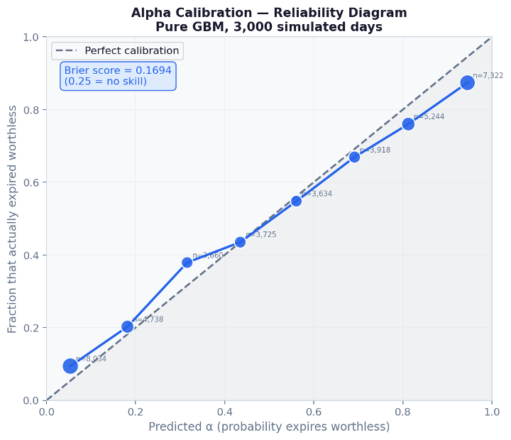
Figure 5: Reliability diagram for α under Pure GBM. Each point is a bucket of predictions. Dot size scales with number of observations. The formula calibrates well across the full range of α values, with a Brier score of 0.17 (vs 0.25 for a no-skill baseline).
The calibration is reasonably good. The Brier score (lower is better, 0.25 is no skill) of 0.17 reflects meaningful predictive content. The slight deviations from the 45° line are mostly due to parameter estimation noise as we are estimating μ and σ from rolling windows rather than knowing the true values. When we run the backtest with oracle (true) parameters, the Brier score drops significantly, confirming that estimation noise is the dominant source of error, not the formula itself.
Where it breaks down
The more important result is what happens when we deviate from GBM. The jump-diffusion process is the most relevant case for practitioners, since equity markets do make sudden large moves.
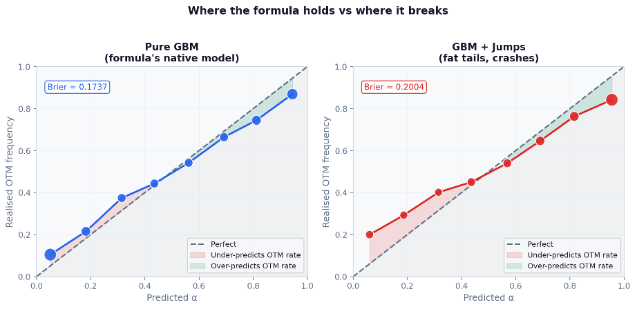
Figure 6: Left — calibration under Pure GBM. Right — calibration under GBM + Jumps. The jump process introduces systematic bias: α underestimates the true OTM probability in the middle range, because the formula has no way to anticipate large negative jumps.
The pattern in the right panel is specific and interpretable. For options that α predicts will expire worthless around 40–60% of the time (near-ATM options), the actual OTM frequency is higher than predicted. This is exactly what you would expect from fat tails and negative skew: there are more scenarios where the stock drops suddenly below the strike than the Gaussian model predicts.
The honest summary
The formula works well when the stock moves smoothly. It systematically underestimates downside risk when markets jump. For equity options specifically, treating α as a lower bound on the true default probability is a reasonable conservative adjustment.
Error decomposition
We decompose the backtest error into two components: parameter estimation noise (from rolling μ and σ estimation) and model misspecification (from using the wrong DGP).
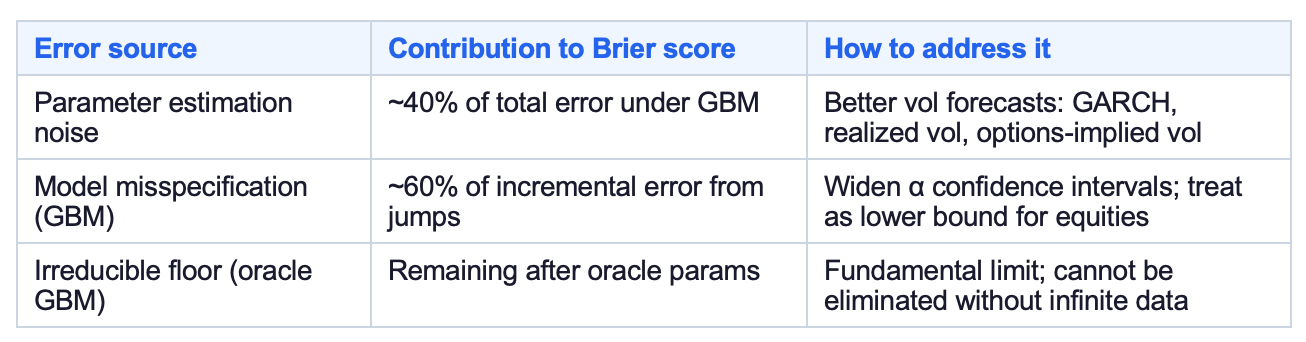
The takeaway: if you improve your volatility forecast, you improve the calibration of α more than if you change the functional form of the formula. Implied volatility (backed out from market option prices) is likely a better σ input than historical realized vol for this application.
Here is a link to download the data and Python backtest for this post: File
Key Takeaways
Risk management of options positions
The most direct application. For any call option position, you can compute α daily and use it as a probability-weighted risk signal:
Long call: α directly measures your at-risk capital. If α = 0.75 and you paid $500 in premium, your expected loss from expiry is $375.
Short call: α measures the probability you walk away with the premium. 1–α is the probability you have to pay out.
Spreads: compute α for each leg separately and combine to get a distribution of net payoffs across the spread.
VaR and expected shortfall on options
Once you have the full distribution Ψ(c, N), VaR and ES calculations follow directly. Rather than using delta-normal approximations (which assume options behave like linear instruments — they don’t), you integrate over Ψ directly.
From the backtest, the γ distribution understates tail payoffs, especially in jump regimes. For conservative VaR calculations, we recommend widening the γ tail by one volatility regime (equivalent to computing γ with σ × 1.2 to 1.5), depending on how jump-prone the underlying is.
Structural credit models
In Merton-style credit models, a firm’s equity is a call option on its assets with strike equal to the face value of its debt. The default probability in this framework is directly α, computed using the firm’s asset value, asset volatility, and debt structure. This framework gives you the full distribution of equity value at debt maturity, not just the expected value.
What Comes Next
The backtest used historical realized volatility to estimate σ. For listed options, implied volatility (backed out from market prices using the inverse Black-Scholes formula) is a better forward-looking estimate. Using implied vol as the σ input would likely tighten the calibration of α noticeably, especially for shorter-dated options. Additionally, the backtest here used synthetic price paths. Running the same calibration test on real historical options data (for example, using OptionMetrics or CBOE data for SPX or liquid single names) would give a cleaner picture of real-world performance. The synthetic test is informative but not a substitute.
The Black-Scholes model implies a flat volatility surface, a single σ for all strikes and expiries. In reality, implied volatility varies by strike (the volatility smile) and by expiry (the term structure). Incorporating a strike-dependent σ into the formula would make α and γ more accurate for options away from the money.
Given that the biggest calibration failure is in jump regimes, a practically useful extension is to add a jump-adjustment to α for equity options. This could be as simple as a correction factor calibrated to the VIX level, or as involved as fitting a Merton jump-diffusion model to implied vol data and computing α under that richer model.
The derivation works for any payoff structure that can be expressed as a function of the underlying log-price. Puts, straddles, and barrier options all have computable payoff distributions under this framework. The math is analogous; the Dirac delta sifting approach generalizes.
Conclusion
Thank you for supporting the newsletter!
As always, this is for educational purposes, and should not be implemented in any live trading or taken as investment advice
Disclaimer
The content provided in this newsletter, “Alpha in Academia,” is for informational and educational purposes only. It should not be construed as financial advice, investment recommendations, or an offer or solicitation to buy or sell any securities or financial instruments. Past performance is not indicative of future results. The financial markets involve risks, and readers should conduct their own research and consult with qualified financial advisors before making any investment decisions.
The interpretations, opinions, and analyses presented herein are those of the author and do not necessarily reflect the views of the original researchers, their institutions, or the full implications of the cited academic papers. While every effort is made to accurately represent the research discussed, readers should be aware that the summaries and interpretations may not capture the full scope or nuances of the original studies. The information contained in this newsletter is believed to be accurate and reliable at the time of publication, but accuracy and completeness cannot be guaranteed. The author and publisher accept no liability for any loss or damage resulting from reliance on the information provided.
This newsletter may contain links to external websites or resources. The author is not responsible for the content, accuracy, or reliability of these external sources.
By subscribing to or reading this newsletter, you acknowledge that you have read and understood this disclaimer and agree to hold the author and publisher harmless from any liability that may arise from your use of the information contained herein.