

Hello and welcome back to another paid post!
Part 1 of 2. This piece sets up the measurement and asks what a published anomaly was doing in the decades before its own paper's sample begins. Part 2 takes the post-publication drop that falls out of it and tests whether that drop is an arbitrage effect at all.
Today we are looking at what happens to a published stock market anomaly across its life. Across 210 anomalies from the academic literature, the long-short return inside each paper’s own sample averages 0.671% a month. Outside that window it averages roughly half as much, and it does not much matter which direction you look. Before the anomaly was discovered, 0.402%. After it was published, 0.334%.
Those two out-of-sample figures are not distinguishable from one another. A formal test of the difference between them returns a z-statistic of 1.04 and a p-value of 0.299, which is nowhere near rejecting equality. The decay from in-sample is large and it is robust. What it is not is something that happened at publication, because the same shortfall is already sitting there in data from decades earlier.
Let’s dive right in.
Introduction
The standard account of anomaly decay runs through arbitrage. An academic finds a predictable pattern in returns, publishes it, practitioners read the paper and trade the signal, and the excess return gets competed away. McLean and Pontiff put hard numbers on this in 2016. Across 97 predictors, portfolio returns were 26% lower out-of-sample and 58% lower after publication, and they attributed the 32-point gap between those to investors learning about mispricing from the academic literature.
The mechanism is sensible and the decay is easy to verify. The part that gets less attention is the counterfactual. If you want to know what publication did to an anomaly, you need a period where the anomaly was measurable but had not been selected, and there are two such periods rather than one. There is the obvious one after the paper comes out. There is also a much longer one before the paper’s sample even begins.
It is worth being precise about why that second period counts as out-of-sample, because there is an obvious objection. All of this is a backtest. The authors were themselves running a backtest when they wrote the paper. So what exactly separates their window from mine?
The answer is selection, not trading. The authors chose that signal, that sort, those breakpoints, and that sample because the combination worked in the window they examined. Every one of those choices is a degree of freedom, and every one was exercised against in-sample data. The pre-discovery window was never part of the search space. It is out-of-sample in exactly the way a holdout period is out-of-sample, and the fact that nobody was trading on it is beside the point. Some practitioners may well have been trading these signals before the papers appeared, and I have no way of knowing. What I can say is that the specification search that produced the published result never saw this data.
In plain terms. If you try enough variations of a trading rule against the same stretch of history, one of them will look excellent whether or not it means anything. The only way to separate a real edge from a lucky variation is to run it on data you never touched while choosing. The decades sitting before each paper's sample are exactly that data, and nobody has to have been trading on them for that to be true.
Linnainmaa and Roberts made this argument in the Review of Financial Studies in 2018. They hand-collected accounting data from Moody’s manuals back to 1918 so they could measure 36 anomalies before their discovery, and they found that the pre-discovery and post-discovery periods resemble each other while the in-sample period resembles neither. Their conclusion was that most accounting-based anomalies are largely a data-snooping artifact.
I wanted to run that design on a much wider set of anomalies, with portfolio construction that follows each original paper rather than a standardized factor build, and with the nine additional years of returns that have accumulated since they wrote.
Data and Methodology
Everything comes from the Open Source Asset Pricing project, the October 2025 release. Chen and Zimmermann replicate the cross-sectional asset pricing literature and publish both the signals and the resulting portfolios, and the project exists to be used and cited rather than licensed.
The dataset gives 212 predictors with monthly long-short returns from January 1926 to December 2024, built the way each original paper built them. I use that construction rather than a house-standard decile sort deliberately. The question is what happened to the strategy each paper actually published, not to a re-specified version of it.
The accompanying documentation file is what makes the design possible. For every anomaly it records the publication year, the journal, the start and end years of the original study’s sample, and the return and t-statistic the authors reported. Publication years run from 1973 to 2016. Original samples end between 1968 and 2014.
From those two dates I cut each anomaly’s return history into four regimes on its own clock. Everything before the paper’s sample begins is pre-discovery. The paper’s own sample window is in-sample. Everything from the end of that sample up to publication is the post-sample window. Everything after publication is post-publication.
The gap between sample end and publication is what makes this design work. It is never zero in this dataset. The minimum is two years, the median is four, the maximum is eleven. That window is a period when the anomaly’s most recent behavior was unknown to its own authors and unknown to everyone else, which separates two explanations that otherwise get confounded. Decay that shows up there cannot be arbitrage, because there was nothing to arbitrage yet. It has to be overfitting.
In plain terms. Every anomaly gets a timeline with four stretches: the long run-up before its paper's data even starts, the paper's own window, a short gap after that window closes but before the paper appears, and everything since. The short gap is the useful one. Nobody outside the authors knew about the finding yet, so anything that falls away there is the original result being flattered by its own sample rather than traders competing it away.
Two choices are worth stating. I treat a paper published in year Y as becoming public on 31 December of Y, which assigns the whole publication year to the pre-publication side. That is the conservative direction, as it biases the design against finding a publication effect. And I require at least 24 months in each of the three regimes the main regression uses, which drops two of the anomalies.
Regressions are pooled across anomalies and months with standard errors clustered by calendar month. That correction matters here more than it usually does. These 210 strategies hold overlapping positions in the same stocks and move together, and treating their monthly returns as independent observations would make everything look far more significant than it is.
Here is what the design looks like on four anomalies you will recognize.
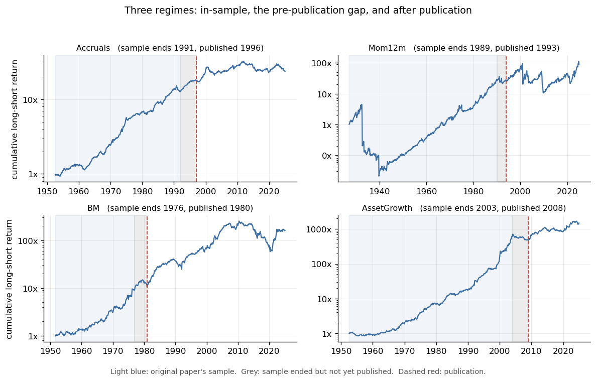
Figure 1: Cumulative long-short returns for four familiar anomalies, with each one's regimes shaded on its own clock. Light blue is the paper's own sample. Grey is the window after that sample ended but before the paper appeared. The dashed red line is publication.
Results
Taking in-sample as the reference, pre-discovery averages 0.402% a month, which is 0.269 percentage points lower with a t-statistic of −4.58. The post-sample window averages 0.424%, down 0.247 at t=−3.77. Post-publication averages 0.334%, down 0.338 at t=−6.56. In-sample itself is 0.671%.
Total decay from in-sample to post-publication is 50.3%. About three quarters of that, 36.9 percentage points, is already present in the post-sample window, before anyone outside the authors could have read the paper.
Those two numbers are directly comparable to McLean and Pontiff, and the comparison is informative. Their out-of-sample decline was 26% against my 36.9%, and their post-publication decline was 58% against my 50.3%. So I find more decay before publication than they did and less after it, which leaves a residual of 13.4 points where they found 32.
The comparison that carries this post, though, is between the two out-of-sample periods. Pre-discovery minus post-publication is +0.069 percentage points with a z-statistic of 1.04 and a p-value of 0.299. Whatever an anomaly earned in the decades before its discovery, it earned about the same after everybody had read about it, and the difference between those two is well inside noise.
The in-sample window is the outlier. Step outside it in either direction and you get roughly half the advertised number.
In plain terms. The average anomaly earned about 0.67% a month in the window its discoverers examined and somewhere between 0.33% and 0.42% everywhere else. Whether “everywhere else” means the forty years before the paper or the twenty years after it makes almost no difference. Roughly half the advertised return was a property of the window rather than of the strategy.
I have deliberately left the arbitrage question out of this post. That 0.338 post-publication coefficient looks like an arbitrage effect, and establishing whether it is one takes more space than I have here. It is the subject of Part 2.